The ancient Phoenicians were great traders and sea farers, but they tended to overload their boats. In stormy weather, goods had to be thrown overboard in order to save the ship. Owners of lost goods were then compensated by those who did not lose their goods, and the amounts involved depended on the total value of the goods. This arrangement was named havara, and this term evolved over the centuries to become average, and from average the mathematical term mean developed.

The astronomer, Gauss, measured distances between stars. He noticed that it was difficult to reproduce his measurements exactly. However, the measurements clustered around a central value, more common near the mean, and becoming less common as they are further away from the mean (fig. left).

He concluded that any set of measurements would normally distribute to this pattern and called it the Normal Distribution.

De Moivre derived the formula for the Normal Distribution curve in mathematical terms (fig. right).

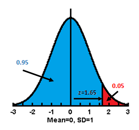
Once this was done, the features of Normal Distribution could be mathematically handled. Using simple calculus, the area under the curve (or any part of it) can be estimated. Fisher developed the concept further and used the area under the curve as a measure of probability. He argues that if the area under the whole curve be consider totality, then any portion represents the probability of the events that describe the portion. From this, he was able to calculate the probability of obtaining a measurement that exceeds a deviation from the mean value. He standardized the measurement of this deviation and called it the Normal Standard Deviate (z), later abbreviated to Standard Deviation, and derived the relationships between z and probability.

The other panels of this page are

• Calculations: Javascript program to calculate the probability of z
• Table: Table of probability of z
• Codes: R and Python codes for calculation of z

References

https://home.ubalt.edu/ntsbarsh/business-stat/StatistialTables.pdf Tables of probability values

https://en.wikipedia.org/wiki/Standard_normal_table Wikipedia explanation and tables
Javascript algorithm adapted from Abramowitz M and Stegun IA (1972) Handbook of mathematical functions. Dover Publications, Inc. New York. Library of Congress Catalog card number 65-12253. p.925

Data	Data = rows of values for z or probability

Calculation are presented in maroon and results produced presented in navy

R Code

Probability of z

ZToP<-function(z)               #function to calculate probability from z
{
  return (1-pnorm(z))
}
ZToP(1.65)                      # testing

0.04947147

PToZ<-function(p)               #function to calculate z from probability
{
    return (-qnorm(p))
}
PToZ(0.05)                      # testing

1.644854

Python Code

Header and Library

import scipy.stats as st

Probability of z

def ZToP(z):
    """ Calculate probability from z """
    return 1 - st.norm.cdf(z)
print(ZToP(1.64))                    # testing

0.050502583474103746

def PToZ(p):
    """ Calculate z from probability """
    return st.norm.ppf(1 - p)
print(PToZ(0.05))                    # testing

1.6448536269514722

The z value is the sum of the first row and first column, and probability is the cell of that row and column. for example, probability=0.40905 when z=0.23

Please be reminded that, although probabilities of z are presented to 5 decimal points of precision in the table, only a 2-4 decimal point precisions are more commonly used.

	0.00	0.01	0.02	0.03	0.04	0.05	0.06	0.07	0.08	0.09
0.0	0.50000	0.49601	0.49202	0.48803	0.48405	0.48006	0.47608	0.47210	0.46812	0.46414
0.1	0.46017	0.45620	0.45224	0.44828	0.44433	0.44038	0.43644	0.43251	0.42858	0.42465
0.2	0.42074	0.41683	0.41294	0.40905	0.40517	0.40129	0.39743	0.39358	0.38974	0.38591
0.3	0.38209	0.37828	0.37448	0.37070	0.36693	0.36317	0.35942	0.35569	0.35197	0.34827
0.4	0.34458	0.34090	0.33724	0.33360	0.32997	0.32636	0.32276	0.31918	0.31561	0.31207
0.5	0.30854	0.30503	0.30153	0.29806	0.29460	0.29116	0.28774	0.28434	0.28096	0.27760
0.6	0.27425	0.27093	0.26763	0.26435	0.26109	0.25785	0.25463	0.25143	0.24825	0.24510
0.7	0.24196	0.23885	0.23576	0.23270	0.22965	0.22663	0.22363	0.22065	0.21770	0.21476
0.8	0.21186	0.20897	0.20611	0.20327	0.20045	0.19766	0.19489	0.19215	0.18943	0.18673
0.9	0.18406	0.18141	0.17879	0.17619	0.17361	0.17106	0.16853	0.16602	0.16354	0.16109
	0.00	0.01	0.02	0.03	0.04	0.05	0.06	0.07	0.08	0.09
1.0	0.15866	0.15625	0.15386	0.15151	0.14917	0.14686	0.14457	0.14231	0.14007	0.13786
1.1	0.13567	0.13350	0.13136	0.12924	0.12714	0.12507	0.12302	0.12100	0.11900	0.11702
1.2	0.11507	0.11314	0.11123	0.10935	0.10749	0.10565	0.10383	0.10204	0.10027	0.09853
1.3	0.09680	0.09510	0.09342	0.09176	0.09012	0.08851	0.08691	0.08534	0.08379	0.08226
1.4	0.08076	0.07927	0.07780	0.07636	0.07493	0.07353	0.07214	0.07078	0.06944	0.06811
1.5	0.06681	0.06552	0.06426	0.06301	0.06178	0.06057	0.05938	0.05821	0.05705	0.05592
1.6	0.05480	0.05370	0.05262	0.05155	0.05050	0.04947	0.04846	0.04746	0.04648	0.04551
1.7	0.04457	0.04363	0.04272	0.04182	0.04093	0.04006	0.03920	0.03836	0.03754	0.03673
1.8	0.03593	0.03515	0.03438	0.03363	0.03288	0.03216	0.03144	0.03074	0.03005	0.02938
1.9	0.02872	0.02807	0.02743	0.02680	0.02619	0.02559	0.02500	0.02442	0.02385	0.02330
	0.00	0.01	0.02	0.03	0.04	0.05	0.06	0.07	0.08	0.09
2.0	0.02275	0.02222	0.02169	0.02118	0.02068	0.02018	0.01970	0.01923	0.01876	0.01831
2.1	0.01786	0.01743	0.01700	0.01659	0.01618	0.01578	0.01539	0.01500	0.01463	0.01426
2.2	0.01390	0.01355	0.01321	0.01287	0.01255	0.01222	0.01191	0.01160	0.01130	0.01101
2.3	0.01072	0.01044	0.01017	0.00990	0.00964	0.00939	0.00914	0.00889	0.00866	0.00842
2.4	0.00820	0.00798	0.00776	0.00755	0.00734	0.00714	0.00695	0.00676	0.00657	0.00639
2.5	0.00621	0.00604	0.00587	0.00570	0.00554	0.00539	0.00523	0.00508	0.00494	0.00480
2.6	0.00466	0.00453	0.00440	0.00427	0.00415	0.00402	0.00391	0.00379	0.00368	0.00357
2.7	0.00347	0.00336	0.00326	0.00317	0.00307	0.00298	0.00289	0.00280	0.00272	0.00264
2.8	0.00255	0.00248	0.00240	0.00233	0.00226	0.00219	0.00212	0.00205	0.00199	0.00193
2.9	0.00187	0.00181	0.00175	0.00169	0.00164	0.00159	0.00154	0.00149	0.00144	0.00139
	0.00	0.01	0.02	0.03	0.04	0.05	0.06	0.07	0.08	0.09
3.0	0.00135	0.00131	0.00126	0.00122	0.00118	0.00114	0.00111	0.00107	0.00103	0.00100
3.1	0.00097	0.00094	0.00090	0.00087	0.00084	0.00082	0.00079	0.00076	0.00074	0.00071
3.2	0.00069	0.00066	0.00064	0.00062	0.00060	0.00058	0.00056	0.00054	0.00052	0.00050
3.3	0.00048	0.00047	0.00045	0.00043	0.00042	0.00040	0.00039	0.00038	0.00036	0.00035
3.4	0.00034	0.00032	0.00031	0.00030	0.00029	0.00028	0.00027	0.00026	0.00025	0.00024
3.5	0.00023	0.00022	0.00022	0.00021	0.00020	0.00019	0.00019	0.00018	0.00017	0.00017
3.6	0.00016	0.00015	0.00015	0.00014	0.00014	0.00013	0.00013	0.00012	0.00012	0.00011
3.7	0.00011	0.00010	0.00010	0.00010	0.00009	0.00009	0.00009	0.00008	0.00008	0.00008
3.8	0.00007	0.00007	0.00007	0.00006	0.00006	0.00006	0.00006	0.00005	0.00005	0.00005
3.9	0.00005	0.00005	0.00004	0.00004	0.00004	0.00004	0.00004	0.00004	0.00003	0.00003

Probability	z value
0.20	0.85	power=0.8, β=0.2
0.10	1.29
0.05	1.65	statistical significane p<0.05
0.025	1.96	95% confidence interval (2.5% each side)
0.01	2.33
0.005	2.58
0.0025	2.81
0.001	3.10