Introduction

The standard decision making in statistical analysis is to define an adequate sample size, collect the data, and draw conclusions based on the data. Sequential analysis does not pre-define a sample size. Rather, it draws decision lines, then analyses the data as it is collected, and draws conclusions when the decision borders are crossed.

Sequential analysis is often attractive, as conclusions can be drawn with a smaller sample size if the outcome is clear and obvious. However, because of the frequent examination of the data, the required sample size can be larger than the fixed sample size model if the outcome is ambiguous.

This page presents the Sequential Probability Ratio Test (SPRT). This is the earliest sequential method, developed by Wald, Neyman, and Pearson and their group during the 1930s. These methods were initially developed as a method of quality control, and they form the basis of many subsequent and more sophisticated developments in sequential and quality control methodologies.

The model aims to determine the quality of a batch of products by minimal sampling. The idea is to sample the batch sequentially until a decision can be made whether the batch conforms to specification and can be accepted, or that the specification is significantly violation and the batch should be rejected.

Common Terms and Abbreviations

• α : , also represented as alpha, or p, is the probability of Type I Error. Commonly, p<0.05 or p<0.01 is used as the criteria to reject the null hypothesis
• β : is the probability of Type II Error. Commonly, β<0.2 is used at the planning stage to determine sample size or calculating borders for sequential analysis.
• Power : is 1 - β, a concept intuitively easier to understand, and represents the ability to detect a difference, if its really there. A power of 0.8 (80%) is usually used as this is the same as β=0.2
• Value to accept null hypothesis : is the lower value (proportion or mean) below which the decision to accept the null hypothesis (not significantly different from zero) can be made.
• Value to reject null hypothesis : is the higher value (proportion or mean) above which the decision to reject the null hypothesis (significantly different from zero) can be made.
• k : was used by Wald to represent the effect size, and is equivalent to θ which is now more commonly used.
• Decision borders : are two parallel lines drawn on the sequential chart. Data are plotted as they are sampled. Sampling continues while the plot coordinates are between the two decision lines. Sampling stops when the plot coordinates are outside of the two lines. If it is above the rejection line then the null hypothesis is rejected. If it is below the acceptance line then the null hypothesis is accepted.
• Truncation : This is the maximum number of samples. Sampling stops at this point even if the coordinate still fall between the two lines. The null hypothesis is usually then accepted. In some algorithms (such as that on these pages, Lines are drawn between the two borders to a midpoint at truncation, and the decision to reject or accept the null hypothesis is made according to which line the last data point crosses.

Sequential Probability Ratio Test (SPRT) for a mean

Data Input : In addition to α and power that are common inputs to both models, the following inputs are used

• Standard Deviation is the expected Standard Deviation of the samples to be taken. In quality control this value is usually known from past history
• Mean (accept null hypothesis): is the mean value below which a decision that the mean is null (zero) can be made. In quality control, to detect defects in production, this is the mean of departure from expected measurements that can be accepted as normal variations.
• Mean (reject null hypothesis): is the mean value above which a decision that the mean is not null (zero) can be made. In quality control, to detect defects in production, this is the mean value of departure from expected values which will trigger an alert that something is amiss.

Example:

1.4
1.1
0.7
0.2
1.3
1.4
1.2
2.0
0.3
0.1
1.4
1.2
0.3
1.1
0.5

The following example is used to demonstrate the program.

We purchase ball bearings in batches in our manufacturing business. Each batch is inspected to make sure the quality complies with our needs.

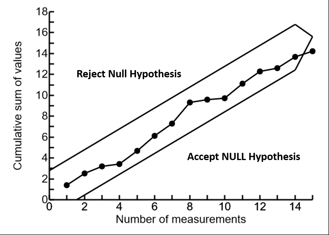
The ball bearing should be 1cm in diameter, with an expected Standard Deviation of 1mm. We decided thst if the average departure from 1cm is less than 0.5 mm, we will accept the batch. However if the departures are greater than 1.5mm, we will reject the batch. We will use α=0.05 and power of 0.8 for testing.

From the parameters, the decision borders can be drawn. Each batch is then randomly sampled, and the cumulative departure from 1 cm plotted and compared with the borders.

The testing for a batch is shown in this example. The departure from 1cm in the samples are as shown in the column to the right. The plot for decision borders and the cumulative sum of departures are shown in the diagram to the left

It can be seen, on the 15th sample, the cumulative sum line crossed the lower acceptance border. The sampling therefore can stop, and the batch accepted as conforming to specifications.

Sequential Probability Ratio Test (SPRT) for a proportion

0
0
0
0
0
0
0
0
1
0
0
0
0
0
0
0
0
0
0
0
0
0
0
1
0
0
0
0
0
1

Data Input : In addition to α and power that are common inputs to both models, the following inputs are used

• Proportion (accept null hypothesis) p0: is the proportion of positives below which a decision that the proportion is null (zero) can be made. In quality control, to detect defective items in a batch of products, this is the proportion of defectives below which the batch can be accepted by the client.
• Proportion (reject null hypothesis) p1: is the proportion of positives above which a decision that the proportion is not null (zero) can be made. In quality control, to detect defective items in a batch of products, this is the proportion of defectives above which the batch will not be accepted by the client.

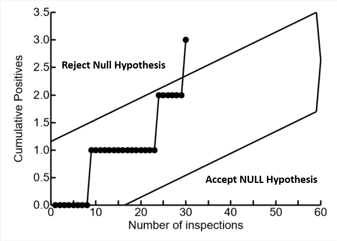
Example: We will quality control the shape of the ball bearings we purchased using SPRT for proportions.

The ball bearings are sampled for defects. We decided that we will rejct the batch if the defective rate exceeds 10% (0.1), and accept the batch if the defective rate is less than 1% (0.01). We will use α=0.05 and power=0.8

The decision borders can be drawn using the parameters. The cumulative number of defective items can then be ploted and compared to the border. The column to the right shows the results of random sampling, 0=non-defective and 1=defective. The diagram to the left shows the borders and the cumulative number of defective items samples from a batch

It can be seen that the line for cumulative number of defective ball bearings crosed the rejection line at the 30th sample, when the third defective item was found. At that point sampling can stop, and the batch rejected as having more defective items than specified.

References

Wald A (1947) Sequential Analysis. John Wiley & Son, Inc, New York. (Original book)

https://ia601603.us.archive.org/11/items/in.ernet.dli.2015.510091/2015.510091.Sequential-Analysis.pdf Wald's book as pdf file on internet archive

https://en.wikipedia.org/wiki/Sequential_probability_ratio_test is a complete and excellent explanation of Wald's SPRT, including the formulae used.

Data

Sequential Mean Sequential Proportion C D E Data: a single column of meaaurement values Parameters: Probability of Type I Error (alpha) Power (1 - beta) Standard Deviation Mean(accept null hypothesis) Mean(reject null hypothesis) Data: a single column of 0 for negatives or 1 for positives Parameters: Probability of Type I Error (alpha) Power (1 - beta) Proportion(accept null hypothesis) Proportion(reject null hypothesis) Contents of C:12 Contents of D:13 Contents of E:14

MacroPlot Code

This panel provides R codes for the two Sequential Probability Ratio Tests (SPRT)

SPRT for mean

# Pgm 1: SPRT for means
# Parameters
alpha = 0.05     # Probability of Type I Error (α)
power = 0.8      # power (1 - β)
sd = 1.0         # Expected Standard Deviation of the measurement
reject = 1.5     # mean of measurements for rejecting null hypothesis (exceed tolerable error)
accept = 0.5     # mean of measurements for accepting null hypothesis (within tolerable error)
# data entry     # Sequence of measurements
arVal <- c(1.4,1.1,0.7,0.2,1.3,1.4,1.2,2.0,0.3,0.1,1.4,1.2,0.3,1.1,0.5) # values

# calculations    
rows = length(arVal)            # sample size
beta = 1 - power                # Probability of Type II Error β
top = -log(beta / (1.0 - alpha)) * log((1 - beta) / alpha)
bot = (reject - accept)^2
n = ceiling(top / bot * sd^2)                 # expected sample size x 3
xend = n * 3                                  # truncated for sequential testing
maxx = xend                                   # max x for plotting
if(rows>maxx) maxx = rows;
# Coefficients
s = (accept + reject) / 2.0                                # slope of decision border
h0 = sd^2 / (reject - accept) * log(beta / (1.0 - alpha))  # constant for acceptance border
h1 = sd^2 / (reject - accept) * log((1.0 - beta) / alpha)  # constant for rejecton border

# Create vectors for plotting decision borders
# rejection line
rejX <- c(0, (xend - 1))                                 # rejection line x1, x2
rejY <- c(h1, (h1 + s * (xend - 1)))                     # rejection line y1, y2
maxy = rejY[2]                                           # max y for plot
# acceptance line
#xstart = 0
#if (h0<0){ xstart = abs(h0 / s) }                        # accptance line begins where y=0
#xstart = 0
xstart = abs(h0 / s)                                     # accptance line begins where y=0
accX <- c(xstart, (xend - 1))                            # acceptance line x1, x2
accY <- c(0, (h0 + s * (xend-1)))            # acceptance line y1, y2
# Extension of decision border beyund truncation if no decision at truncation
y1X <- vector()
y1Y <- vector()
y2X <- vector()
y2Y <- vector()
y3X <- vector()
y3Y <- vector()

y1 = h1 + s * (xend - 1)
y2 = h0 + s * (xend - 1)
y3 = (h1 + h0) / 2 + s * xend
y1X <- c((xend-1), xend)            # x1, x2 for rejection line converging towards average with acceptance line
y1Y <- c(y1, y3)              # y1, y2 for rejection line converging towards average with acceptance line
y2X <- c((xend-1), xend)            # x1, x2 for acceptance line converging towards average with rejection line
y2Y <- c(y2, y3)              # y1, y2 for acceptance line converging towards average with rejection line
if(rows>xend)          #  Single decision line following end of truncation           
{
  y3X <- c(xend, rows)                         # x1, x2 for single decision line
  y3Y <- c(y3, ((h1 + h0) / 2 + s * rows))  # y1, y2 for single decision line
}

# Create data plotting array
arX <- vector()                     # x values, number of observations
arY <- vector()                     # y value, cumulative sum of measurements
cusum = 0
for(i in 1 : length(arVal))
{
  arX <- append(arX,i)
  cusum = cusum + arVal[i]
  arY <- append(arY,cusum)
}
y = arY[length(arY)]
if(y>maxy){maxy = y}                #arX# adjust max y for plotting

# Output results of calculations
c(rows, xend)       # sample size and end of plot
c(s, h0, h1)        # slope, constant(accept) , constant (reject) of decision border

The initial output of the decision borders are as follows

> # Output results of calculations
> c(rows, xend)       # sample size and end of plot
[1] 15 15
> c(s, h0, h1)        # slope, constant(accept) , constant (reject) of decision border
[1]  1.000000 -1.558145  2.772589

Plotting: The decision borders and the cumulative sums are plotted as follows

# plot all calculations
par(pin=c(4.2, 3))    # set plotting window to 4.2x3 inches
plot(
  xlim = c(0,maxx),
  ylim = c(0,maxy),
  x   = arX,                 # x = n observations
  y   = arY,                 # y = cum sum
  type = "b",
  pch = 16,                        # size of dot
  xlab = "Number of Measurements", # x label
  ylab = "Cumulative Sum")         # y lable
#lines(arX, arY)                 # line joining dots 
lines(rejX, rejY)               # rejection line
lines(accX, accY)               # acceptance line line
lines(y1X, y1Y)                 # reject tail
lines(y2X, y2Y)                 # accept tail
lines(y3X, y3Y)                 # beyound tail

This results in the plot to the right

Program 2: SPRT for proportion

# Program 2: SPRT proportions
# parameters
alpha = 0.05     # Probability of Type I Error ??
power = 0.8      # power (1 - ??)
accept = 0.01    # proportion for accepting null hypothesis (within tolerable error)
reject = 0.1     # proporiion for rejecting null hypothesis (exceed tolerable error)
arVal <- c(0,0,0,0,0,0,0,0,1,0,0,0,0,0,0,0,0,0,0,0,0,0,0,1,0,0,0,0,0,1) # 0=negative 1 = positive
# calculations
rows = length(arVal)                                                # sample size
beta = 1 - power                                                    # probability of Type II error ??
top = -log(beta / (1.0 - alpha)) * log((1 - beta) / alpha)
bot = log(reject / accept) * log((1.0 - accept) / (1.0 - reject))
n = ceiling(top / bot)                                          # expected truncation for decisions
xend = n * 3;
maxx = xend
if(rows>maxx){ maxx = rows}      
# adjusted to sample size
k = log((reject * (1.0 - accept)) / (accept * (1.0 - reject)))
s = log((1.0 - accept) / (1.0 - reject)) / k
s                                                     # slope of decision border 
h0 = -log((1.0 - alpha) / beta) / k                    # constant for acceptance line
h1 = log((1.0 - beta) / alpha) / k                    # constant for rejection line
rejX <- c(0, (xend - 1))                              # rejection line x1, x2
rejY <- c(h1, (h1 + s * (xend - 1)))                  # rejection line y1, y2
maxy = rejY[2]                                        # max y for plot
# acceptance line

xstart = abs(h0 / s)                                  # accptance line begins where y=0
accX <- c(xstart, (xend - 1))                         # acceptance line x1, x2
#accY <- c((s * xstart - h0), (s * (xend - 1) - h0))   # acceptance line y1, y2
accY <- c(0, (s * (xend - 1) - h0))   # acceptance line y1, y2
# Extension of decision border beyund truncation if no decision at truncation
y1X <- vector()
y1Y <- vector()
y2X <- vector()
y2Y <- vector()
y3X <- vector()
y3Y <- vector()

y1 = h1 + s * (xend - 1)
y2 = s * (xend - 1) + h0
y3 = (h1 + h0) / 2 + s * xend
y1X <- c((xend-1), xend)      # x1, x2 for rejection line converging towards average with acceptance line
y1Y <- c(y1, y3)              # y1, y2 for rejection line converging towards average with acceptance line
y2X <- c((xend-1), xend)      # x1, x2 for acceptance line converging towards average with rejection line
y2Y <- c(y2, y3)              # y1, y2 for acceptance line converging towards average with rejection line
if(rows>xend)          #  Single decision line following end of truncation           
{
  y3X <- c(xend, rows)                      # x1, x2 for single decision line
  y3Y <- c(y3, ((h1 + h0) / 2 + s * rows))  # y1, y2 for single decision line
}

# plotting array
arX <- vector()
arY <- vector()
cusum = 0
for(i in 1 : length(arVal))
{
  arX <- append(arX,i)               # x = number of observarions
  cusum = cusum + arVal[i]
  arY <- append(arY,cusum)           # y = cumulative sum of numbers with positives
}
y = arY[length(arY)]
if(y>maxy){maxy = y}                 # adjust max y value for plotting

# Output results of calculations
c(rows, xend)       # sample size and end of plot
c(s, h0, h1)        # slope, constant(accept) , constant (reject) of decision border

The initial output of the decision borders are as follows

> # Output results of calculations
> c(rows, xend)       # sample size and end of plot
[1] 30 60
> c(s, h0, h1)        # slope, constant(accept) , constant (reject) of decision border
[1]  0.03974743 -0.64979678  1.15625931

Plotting

# plot all calculations
par(pin=c(4.2, 3))   # set plotting window to 4.2x3 inches
plot(
  xlim = c(0,maxx),
  ylim = c(0,maxy),
  x   = arX,                 # x = n observations
  y   = arY,                 # y = cum sum
  type = "b",
  pch = 16,                        # size of dot
  xlab = "Number of Measurements", # x label
  ylab = "Cumulative Sum")         # y lable
#lines(arX, arY)                 # line joining dots 
lines(rejX, rejY)               # rejection line
lines(accX, accY)               # acceptance line line
lines(y1X, y1Y)                 # reject tail
lines(y2X, y2Y)                 # accept tail
lines(y3X, y3Y)                 # beyound tail

The plot is as shown to the right

Contents of D:3

Contents of E:4

Contents of F:5