Links : Home Index (Subjects) Contact StatsToDo

Introduction Gaussian Binomial Multinomial Ordinal Poisson H I J K Negative Binomial The Generalized Linear Models (GLM) calculate regression coefficients relating a dependent variable to multiple independent variables. The value of the dependent variable is a linear combination of products of coefficient and value of each independent variable, so the model has the same appearence as that of multiple regression or covariance analysis. A particular advantage of the models is that the algorithms can cope with a combination of factors (group names in text) and values (numerical data), as well as dependent variables from a variety of probability distributions. This allows the models to be highly complex, providing the probability distribution of the data is correctly assumed. It is beyond the capability of this page to provide full explanation or web paged based program for GLM, as it is a vast subject, and the calculations complex. R code examples are offered on this page, as these algorithms are already fully developed, tested, and accepted. Only brief explanations, assisting users to negotiate the R codes are offered For those new to using R the page R_Exp provides an introduction and help for installation of the R packages For full explation and exploration of this area of statistics, users are referred to the references as the starting point. Users are also reminded to seek advice and assistance from experienced statisticians if they are new to this area of statistics. Programs The panels of this page provides R codes for regression with the following distributions for the dependent variable Gaussian. Where the dependent variable is normally distributed. This model is also termed General Linear Model, not to be confused with the generic name of all the models presented here the Generalized Linear Models When all the independent variables are factors (group names in text), the results are similar to that produced by the Analysis of Variance When all the independent variables are values (numerical measurements), the results are similar to Multiple Regression When the independent variables are a mixture of factors and values, the results are similar to that of Analysis of Covariance Proportions. Three models of regression for proportions are available Binomial Where the dependent variable is the probabilities in each of two groups (no/yes, false/true) Multinomial, the same as Binomial, except there are more than 2 groups Ordinal, the same as Multinominal, except the groups are ordered Poisson where the dependent variable is a count of events in a defined environment, where the variance is the same value as the count Negative Binomial Where the dependent variable is the Odds Ratio of the number of negative cases per positive case in the two groups. Negative Binomial distribution can also be used generally for count data that fails to conform to the Poisson distribution Format Each program is described in one of the subsequent panels. Each panel containing an introduction and a program template, each in a sub-panel Each program is provided with a set of example data, to demonstrate the procedures. Please note: The research model is deliberately simplistic so the user is not distracted from the computation The data is computer generated and do not represent anything real. The sample size is deliberately small, to make visualization easier. The R code in each program is broken up into its constituent steps, and each step contains Description of the step (in black) The R code (in Maroon) The results from that step (in Navy blue) To re-constituate the whole program, the user should Copy all the codes in Maroon to the source code panel of RStudio, in the same order as in the template. This should include the example data Test run the program to make sure it works Change the example data to the user's own data Repeated cycles of test run and editing the codes (add, delete, and modify) until the required results are produced. References Please note that the R code template contins only the minimum amount of code, and produces only the basic results. Users may want to produce a more complete program, including the many options that are availble with each procedure. References are provided in the Explanation panel of each program for this purpose GLM: Dependent Variable with Gaussian (Normal) Distribution (Analysis of Variance) Explanation R Code C D E This panel provides explanations and example R codes for one of the procedures in Generalized Linear Models (GLM), where the dependent variable is a measurement that is normally distributed (Gaussian). The Gaussian model is sometimes termed General Linear Model, and should not be confused with Generalized Linear Models which described a whole genre of regression methods in different panels of this page. GLM for Gussian distributed values produce results that are nearly the same as that of the Least Square Methods (Regression ans Analysis of Variance). Instead of mathematically partitioning the variance into its components, GLM uses adaptive modelling, fitting the data using numerical approximations. In the GLM for Gaussian distribution model If all the independent variables used are measurements (values), the results are similar to that from Regression or Multiple Regression analysis If All the independent variables are group names (factors), the results are similar to thst from Analysis of Variance If the independent variables are a mix of values and factors, then the results are similar to that from Analysis of Covariance References https://rcompanion.org/rcompanion/e_04.html An R Companion for the Handbook of Biological Statistics by Salvatore S. Mangiafico. 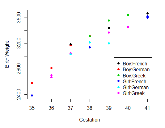Chapter on analysis of covariance https://en.wikipedia.org/wiki/General_linear_model https://en.wikipedia.org/wiki/Generalized_linear_model The example data is computer genrated to demonstrate the computation. It represents a study of birthweight, where the independent variables are sex of the baby (Boy or Girl), ethnicity of the mother (French, German or Greek), and gestational age at birth (weeks), and the dependent variable the weight of the newborn in grams. There are 22 babies (rows) in this set of data. As the independent variables include both factors (sex and ethnicity) and values (gestation), the model is that of Analysis of Covariance The first step is to place the data in a data frame # Step 1: Data entry to dataframe myDat = (" Sex Ethn Gest BWt Girl Greek 37 3048 Boy German 36 2813 Girl French 41 3622 Girl Greek 36 2706 Boy German 35 2581 Boy French 39 3442 Girl Greek 40 3453 Boy German 37 3172 Girl French 35 2386 Boy Greek 39 3555 Girl German 37 3029 Boy French 37 3185 Girl Greek 36 2670 Boy German 38 3314 Girl French 41 3596 Boy Greek 38 3312 Girl German 39 3200 Boy French 41 3667 Boy Greek 40 3643 Girl German 38 3212 Girl French 38 3135 Girl Greek 39 3366 ") myDataFrame <- read.table(textConnection(myDat),header=TRUE) myDataFrame$Sex <- factor(myDataFrame$Sex) # enforce variable as factor myDataFrame$Ethn <- factor(myDataFrame$Ethn) # enforce variable as factor summary(myDataFrame) The summary of the data is as follows > summary(myDataFrame) Sex Ethn Gest BWt Boy :10 French:7 Min. :35.00 Min. :2386 Girl:12 German:7 1st Qu.:37.00 1st Qu.:3034 Greek :8 Median :38.00 Median :3206 Mean :38.05 Mean :3187 3rd Qu.:39.00 3rd Qu.:3450 Max. :41.00 Max. :3667 The second step can be plotting the data # Step 2: Plot Data sx <- factor(myDataFrame$Sex) #abbreviation se <- factor(myDataFrame$Ethn) #abbreviation par(pin=c(4.2, 3)) # set plotting window to 4.2x3 inches plot(x = myDataFrame$Gest, # Gest on the x axis y = myDataFrame$BWt, # BWt on the y axis #col = factor(myDataFrame$Sex):factor(myDataFrame$Ethn), # in 6 colors (sex=2,Ethn=3) col = sx:se, # in 6 colors (sex=2,Ethn=3) pch = 16, # size of dot xlab = "Gestation", # x label ylab = "Birth Weight") # y lable legend('bottomright', # placelegendon bottomright legend = levels(sx:se), #all combinations col = 1:6, # 6 colors for 6groups cex = 1, pch = 16) This step is optional, and included here to provide a template for plotting. It produces a plot of the data. Please note that the names of variables and labels are from the column names of the data, and need to be changed by the user to conform with his/her data set and names The next step is the GLM formula itself, and in this example is divided into two sub-steps Step 3a is optional, and performs analysis of covariance, including a test for interactions # Step 3a: Analysis of variance testing interactions testResults<-aov(BWt~Sex+Ethn+Gest+Sex*Ethn*Gest,data=myDataFrame) #Test for interactions summary(testResults) #show results Analysis of Variance Table The results are in a table of analysis of variance from all sources, shown as follows Df Sum Sq Mean Sq F value Pr(>F) Sex 1 122427 122427 21.300 0.000958 *** Ethn 2 278266 139133 24.206 0.000147 *** Gest 1 2272527 2272527 395.376 2.27e-09 *** Sex:Ethn 2 9208 4604 0.801 0.475688 Sex:Gest 1 4668 4668 0.812 0.388680 Ethn:Gest 2 8719 4360 0.759 0.493517 Sex:Ethn:Gest 2 71921 35960 6.256 0.017292 * Residuals 10 57478 5748 The results of step 3a show significant interaction between Sex, Ethn and Gest. The interpretation is that different combinations of baby's sex and mother's ethnicity have different growth rates. If the data is real, and the sample size sufficiently large, then a more detailed analysis of this interaction is required before proceeding further. As this example data is computer generated, the sample size small, and the intention is to demonstrate the procedures, this significant interaction is ignored, and analysis will proceed to step 3b Step 3b is a repeat of the analysis, but without the interaction terms # Step 3b: Final analysis of variance without interactions aovResults<-aov(BWt~Sex+Ethn+Gest,data=myDataFrame) #analysis of covariance summary(aovResults) #show results Analysis of Variance Table The results are as follows Df Sum Sq Mean Sq F value Pr(>F) Sex 1 122427 122427 13.69 0.001776 ** Ethn 2 278266 139133 15.56 0.000144 *** Gest 1 2272527 2272527 254.18 1.17e-11 *** Residuals 17 151994 8941 This is a standard table of Analysis of variance. It shows that all 3 independent variables contributed significantly to values of birth weight. If these results are accepted, then the next step, step 4, is to establich the formula where birthweight can be predicted from sex, maternal ethnicity and gestation age # Step 4: Generalized Linear Model formula glmResults<-lm(BWt~Sex+Ethn+Gest,data=myDataFrame) # Generalized Linear Model summary(glmResults) #show results Analysis of Variance Table The results are Coefficients: Estimate Std. Error t value Pr(>|t|) (Intercept) -4021.50 467.16 -8.608 1.33e-07 *** SexGirl -165.93 41.07 -4.040 0.000851 *** EthnGerman 58.49 54.91 1.065 0.301682 EthnGreek 77.14 49.75 1.551 0.139430 Gest 190.61 11.96 15.943 1.17e-11 *** The results to focus on is the column under the label Estimates, as this is the formula that models birth weight (BWt) according to Sex, Ethn, and Gestation For factors (groups), unless otherwise assigned, the first group in alphabetical order is the reference group. In this example, Boy comes before Girl, so Boy is the reference group and girls are 165.93g less heavy than boys. For Ethnicity French comes before German or Greeks, so is the reference group. German babies are 58.49g and Greek babies 77.14g heavier than French babies For measurements, the weight is the value x coefficient. This means that babies grows 190.61g per week within the range of this data. The calculations are therefore as follows A French Boy, at 36 week is -4021.5 + 36(190.61) = 2840.46g A girl would weigh 165.93g less A German baby would weigh 58.49g more and a Greek baby 77.14g more For each week after 36 weeks to 42 weeks, the newborn weighs 190.61g more However, there is no need to laboriously calculating and estimate bithweight, as R will perform the task, as in Step 5. This step is optional and for demonstration only. It shows how the results produced can be used to calculate and estimate the value for each case in the dataset. # Step 5: Check that formula works by calculating values and add to dataframe myDataFrame$Fitted<-fitted.values(glmResults) myDataFrame The results are Sex Ethn Gest BWt Fitted 1 Girl Greek 37 3048 2942.461 2 Boy German 36 2813 2899.123 3 Girl French 41 3622 3627.777 4 Girl Greek 36 2706 2751.846 5 Boy German 35 2581 2708.508 .... Step 6 is also optional. It pots the estimated birthweight against the actual bithweight, to show how closely the formula predicts # Step 6: Plot original against calculated par(pin=c(4.2, 3)) # set plotting window to 4.2x3 inches plot(x = myDataFrame$BWt, # Bwt on the x axis y = myDataFrame$Fitted, # Fit on the y axis pch = 16, # size of dot xlab = "Actual Birth Weight", # x label ylab = "Calculated Birth Weight") # y lable x_eq <- function(x){x} #curve function y=x plot(x_eq, 2450, 3700, add=TRUE) #add curve to existing plot The results are shown as follows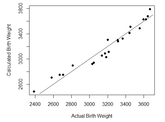 Step 7 demonstrate testing the formula on a new set of data. In 7a, a new data frame is created, consisting of the first 4 rows of the original data. In 7b, the formula produced in step 4 is then used to predict the birth weight # Step 7a: create a new data frame newDat = (" Sex Ethn Gest Girl Greek 37 Boy German 36 Girl French 41 Girl Greek 36 ") # create new dataframe from new input data newDataFrame <- read.table(textConnection(newDat),header=TRUE) summary(newDataFrame) #step 7b: Estimate birthweight from established formula newDataFrame$Model <- predict(glmResults, newdata=newDataFrame, type='response') newDataFrame The results are shown as follows > summary(newDataFrame) Sex Ethn Gest Boy :1 French:1 Min. :36.0 Girl:3 German:1 1st Qu.:36.0 Greek :2 Median :36.5 Mean :37.5 3rd Qu.:38.0 Max. :41.0 > > #step 7b: > newDataFrame$Model <- predict(glmResults, newdata=newDataFrame, type='response') > newDataFrame Sex Ethn Gest Model 1 Girl Greek 37 2942.461 2 Boy German 36 2899.123 3 Girl French 41 3627.777 4 Girl Greek 36 2751.846 Step 7 demonstrate how the results of analysis (glmResults) can be used to estimate birth weight from a different data set. Please note the following The formula in step 5 cannot be use, as it requires that the dataframe has the same name and has the same number of rows as the original data. With the procedure in step 7, a dataframe of different name and different number of rows can be handled. However, the names of the columns used for calculation must still be the same as that from the original dataframe. Step 8 demonstrates how to saves the prediction formula and reload it in future analysis #Step 8: Optional saving and loading of coefficients #save(glmResults, file = "glmResults.rda") #save results to rda file #load("glmResults.rda") #load the rda file The formula is saves as a .rda file, that can be reloaded on a different occasion and used on a different dataset. Please note the following R Studio read and write files using the User/Document/ folder. The path needs to be reset if the user wishes to save and load files using a specific folder. Discussion are in the file I/O panel of the R_Exp.php Once loaded, the conditions for analysis are the same as that in step 7. Contents of C:22 Contents of D:23 Contents of E:24 GLM: Dependent Variable with Binomial Distribution (Probability of a case belonging to one of two Groups) Explanation R Code C D E This page provides explanations and example R codes for Binomial Logistic Regression, where the dependent variable is the probabilities of belonging to one of the two groups. GLM for binomial distribution is also known as Binomial Logistic Regression, or Logistic Regression for short. In this model, the dependent variable y is binomial, one of two outcomes, no/yes, True/false, 0/1. In R, the independent variables can be measurements or factors Measurements are numerical, and can be binary(0/1), ordinal, or parametric Factors are text, and consists of group names. Unless otherwise assigned, R arrange group names alphabetically, and use the first name as the reference group The formula obtained is y = intercept + b1x1 + b2x2 + ....., where b is the coefficient and also the log(odds Ratio) against the reference value. The reference values are 0 for measurement and the reference group for factors. y is then the log odds ratio of outcomes against the reference outcome (outcome name that is alphabetically first) The probability of outcome is then calculated by logistic transform p = 1 / (1 + exp(-y)) References https://en.wikipedia.org/wiki/Logistic_regression Logistic Regression by Wikipedia Cox, DR (1958). "The regression analysis of binary sequences (with discussion)". J Roy Stat Soc B. 20 (2): 215 - 242. JSTOR 2983890. Portney LR, Watkins MP (2000) Foundations of Clinical Research Applications to Practice Second Edition.ISBN 0-8385-2695 0 p. 597 - 603 The example data is computer generated to demonstrate the computation. It perports to be from a study to predict the probability of Caesarean Section (factor of no/yes), based on the height of the mother (value), high blood pressure (factor no/yes), and presence of diabetes (factor 0_No, 1_Mild, 2_Severe) Step 1 consists of creating the data frame from a data set or 5 columns and 22 births (rows) # Step 1: Data entry myDat = (" Parity Diabetes HighBP Height CS Multipara 1_Mild No 157 No Nullipara 0_No Yes 157 No Multipara 0_No No 153 Yes Multipara 2_Severe No 165 No Nullipara 0_No Yes 158 Yes Nullipara 0_No No 158 Yes Multipara 1_Mild No 151 Yes Nullipara 0_No Yes 157 No Multipara 0_No No 163 Yes Nullipara 2_Severe No 163 Yes Multipara 0_No Yes 162 No Nullipara 0_No No 165 No Multipara 1_Mild No 159 No Nullipara 1_Mild Yes 159 Yes Multipara 0_No No 157 Yes Nullipara 2_Severe No 161 Yes Multipara 0_No Yes 156 No Nullipara 0_No No 159 Yes Nullipara 1_Mild No 160 No Multipara 0_No Yes 160 No Multipara 0_No No 158 No Multipara 2_Severe No 160 Yes ") myDataFrame <- read.table(textConnection(myDat),header=TRUE) summary(myDataFrame) The summary of the data is as follows > summary(myDataFrame) Parity Diabetes HighBP Height CS Multipara:12 0_No :13 No :15 Min. :151.0 No :11 Nullipara:10 1_Mild : 5 Yes: 7 1st Qu.:157.0 Yes:11 2_Severe: 4 Median :159.0 Mean :159.0 3rd Qu.:160.8 Max. :165.0 Step 2 is calculating the Binomial Logistic Regression #Step 2: Binomial Logistic Regression binLogRegResults <- glm(CS~Parity+Diabetes+HighBP+Height,data=myDataFrame,family=binomial()) summary(binLogRegResults) The results are as follows > summary(binLogRegResults) Call: glm(formula = CS ~ Parity + Diabetes + HighBP + Height, family = binomial(), data = myDataFrame) Deviance Residuals: Min 1Q Median 3Q Max -1.25281 -0.89430 0.05138 0.62860 1.98546 Coefficients: Estimate Std. Error z value Pr(>|z|) (Intercept) 60.2918 32.4084 1.860 0.0628 . ParityNullipara 1.7912 1.2301 1.456 0.1454 Diabetes1_Mild -1.1484 1.3376 -0.859 0.3906 Diabetes2_Severe 2.0643 1.8111 1.140 0.2544 HighBPYes -2.0810 1.3889 -1.498 0.1340 Height -0.3811 0.2049 -1.860 0.0629 . --- Signif. codes: 0 '***' 0.001 '**' 0.01 '*' 0.05 '.' 0.1 ' ' 1 (Dispersion parameter for binomial family taken to be 1) Null deviance: 30.498 on 21 degrees of freedom Residual deviance: 22.015 on 16 degrees of freedom AIC: 34.015 Number of Fisher Scoring iterations: 5 The results show that none of the independent variables in this analysis has a statistically significant (p<0.05) influence on the outcome. This is not surprising as the data is computer generated and of a very small sample size. The results to focus on are in the column under Estimates which are the coefficients. As an example we will use the fifth row of the data to demonstrate the math Calculation begins with y = intercept = 60.2918 With Parity=Nullipara, y = 60.2918 + 1.7912 With Diabetes=0_No, y = 60.2918 + 1.7912 + 0 With HighBP=Yes, y = 60.2918 + 1.7912 + 0 - 2.0810 With Height = 158, y = 60.2918 + 1.7912 + 0 - 2.0810 - 0.3811(158) y = 60.2918 + 1.7912 + 0 - 2.0810 - 0.3811(158) = -0.2118 which is the log(Odds Ratio) for Caesarean Section (CS:Yes) for this row The probability of CS:Yes is p = Logistic(y) = 1 / (1+exp(-y)) = 0.45 These manual calculations are unnecessary, as R will perform this for you in Step 3, which estimates the probability of Caesareans Section (CS=yes) #Step 3: Calculate probability of outcome using data myDataFrame$Fit<-fitted.values(binLogRegResults) #add predicted probability to dataframe myDataFrame #optional display of dataframe The results are as follows, where the added column fit is the probability of yes for CS > myDataFrame #optional display of dataframe Parity Diabetes HighBP Height CS Fit 1 Multipara 1_Mild No 157 No 0.33558017 2 Nullipara 0_No Yes 157 No 0.54377606 3 Multipara 0_No No 153 Yes 0.87970051 4 Multipara 2_Severe No 165 No 0.37311861 5 Nullipara 0_No Yes 158 Yes 0.44880349 6 Nullipara 0_No No 158 Yes 0.86709292 7 Multipara 1_Mild No 151 Yes 0.83248000 8 Nullipara 0_No Yes 157 No 0.54377606 9 Multipara 0_No No 163 Yes 0.13931363 10 Nullipara 2_Severe No 163 Yes 0.88436769 11 Multipara 0_No Yes 162 No 0.02872213 12 Nullipara 0_No No 165 No 0.31175573 13 Multipara 1_Mild No 159 No 0.19074552 14 Nullipara 1_Mild Yes 159 Yes 0.14995209 15 Multipara 0_No No 157 Yes 0.61428430 16 Nullipara 2_Severe No 161 Yes 0.94249059 17 Multipara 0_No Yes 156 No 0.22537997 18 Nullipara 0_No No 159 Yes 0.81674315 19 Nullipara 1_Mild No 160 No 0.49124223 20 Multipara 0_No Yes 160 No 0.05959019 21 Multipara 0_No No 158 No 0.52106186 22 Multipara 2_Severe No 160 Yes 0.80002311 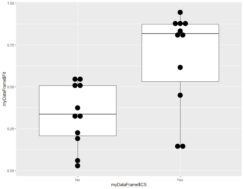Step 4 is optional, a template for frequency plot of the probabilities in the two groups. #step 4: Plot bar and dots of Fitted Probabilities #install.packages("ggplot2") # if not already installed library(ggplot2) ggplot(myDataFrame, aes(x = myDataFrame$CS, y = myDataFrame$Fit)) + geom_boxplot() + geom_dotplot(binaxis="y",binwidth=.03,stackdir="center") The results is in the plot to the left. The data points are circles, the vertical line the range, the horizontal line the mean, and the box the interquartile (25 percentile to 75 percentile) range Stet 5 is to test the formula on a different set of data #Step 5a: Test results on a different set of data newDat = (" Parity Diabetes HighBP Height CS Multipara 1_Mild No 157 No Nullipara 0_No Yes 157 No Multipara 0_No No 153 Yes Multipara 2_Severe No 165 No ") newDataFrame <- read.table(textConnection(newDat),header=TRUE) summary(newDataFrame) #Step 5b: test the model on new data frame newDataFrame$Model <- predict(binLogRegResults, newdata=newDataFrame, type='response') newDataFrame The results are as follows newDat = (" + Parity Diabetes HighBP Height CS + Multipara 1_Mild No 157 No + Nullipara 0_No Yes 157 No + Multipara 0_No No 153 Yes + Multipara 2_Severe No 165 No + ") > newDataFrame <- read.table(textConnection(newDat),header=TRUE) > summary(newDataFrame) Parity Diabetes HighBP Height CS Multipara:3 0_No :2 No :3 Min. :153 No :3 Nullipara:1 1_Mild :1 Yes:1 1st Qu.:156 Yes:1 2_Severe:1 Median :157 Mean :158 3rd Qu.:159 Max. :165 > > newDataFrame$Model <- predict(binLogRegResults, newdata=newDataFrame, type='response') > newDataFrame Parity Diabetes HighBP Height CS Model 1 Multipara 1_Mild No 157 No 0.3355802 2 Nullipara 0_No Yes 157 No 0.5437761 3 Multipara 0_No No 153 Yes 0.8797005 4 Multipara 2_Severe No 165 No 0.3731186 Step 6 is to save the calculated model, and to load it when used subsequently #Step 6: Optional saving and loading of coefficients save(binLogRegResults, file = "binLogRegResults.rda") #save results to rda file load("binLogRegResults.rda") #load the rda file Step 6 is optional, and in fact commented out, and included as a template only. It allows the results of analysis to be stored as a .rda file, that can be reloaded on a different occasion and used on a different dataset. Please note the following R Studio read and write files using the default User/Document/ folder. The path needs to be reset if the user wishes to save and load files using a specific folder. Discussion in the file I/O panel of the R_Exp.php Once loaded, the conditions for analysis are the same as that in step 5. Contents of C:32 Contents of D:33 Contents of E:34 GLM: Dependent Variable with Multinomial Distribution (Probability of more than Two Groups) Explanation R Code C D E Multinomial Logistic Regression is an extension of the Binomial Logistic Regression, as explained in the previous panel, except that the dependent variable has more than two groups. The computation relies on the backpropagation neural network, one with no middle layer, and the transformation function is linear rather than logistic. The interpretation of results however are similar to other Generalized Linear Models In R, the independent variables can be measurements or factors Measurements are numerical, and can be binary(0/1), ordinal, or parametric Factors are text, and consists of group names. Unless otherwise assigned, R arrange group names alphabetically, and use the first name as the reference group The algorithm produces m-1 formulae, m being the number of groups. The probabilities of belonging to the groups are estimated, and the estimated diagnosis assigned to that with the highest probability. Details on how this is carried out are described in the R code panel References https://stats.idre.ucla.edu/r/dae/multinomial-logistic-regression/ https://en.wikipedia.org/wiki/Multinomial_logistic_regression The data is computer generated, and purports to be from a study of admissions from Emergency Department who felt unwell and has abdominal pain. The model is to make a diagnosis between appendicitis (Appen), Urinary Tract Infection (UTI), and the flu (Flu), based on the presence of vomiting (Vomit), the temperature (Temp) and pulse rate (Pulse). Step 1 consists of creating the data frame from a data set or 4 columns and 15 cases (rows) # Step 1: Data entry to dataframe myDat = (" Vomit Pulse Temp Diagnosis No 74 102 Appen Yes 68 97 UTI No 78 99 Flu Yes 72 98 UTI No 72 101 Flu Yes 92 96 Appen No 76 100 UTI No 86 100 Appen No 74 98 Flu No 72 99 UTI Yes 84 100 Flu Yes 85 98 Appen No 64 103 Flu No 78 97 UTI Yes 72 99 Appen ") myDataFrame <- read.table(textConnection(myDat),header=TRUE) summary(myDataFrame) The summary of the input data is shown as follows > summary(myDataFrame) Vomit Pulse Temp Diagnosis No :9 Min. :64.00 Min. : 96.00 Appen:5 Yes:6 1st Qu.:72.00 1st Qu.: 98.00 Flu :5 Median :74.00 Median : 99.00 UTI :5 Mean :76.47 Mean : 99.13 3rd Qu.:81.00 3rd Qu.:100.00 Max. :92.00 Max. :103.00 Step 2:Performing Multinomial Regression # Step 2: Multinomial Logistic Regression #install.packages("nnet") # if not already installed library(nnet) mulLogRegResults <- multinom(formula = Diagnosis ~ Vomit + Pulse + Temp, data = myDataFrame) summary(mulLogRegResults) #display results The results are as follows multinom(formula = Diagnosis ~ Vomit + Pulse + Temp, data = myDataFrame) Coefficients: (Intercept) VomitYes Pulse Temp Flu 21.9547 -1.290127 -0.1272113 -0.1159828 UTI 143.5231 -2.036092 -0.3264960 -1.1910271 Std. Errors: (Intercept) VomitYes Pulse Temp Flu 0.02710540 1.641638 0.1015629 0.07724494 UTI 0.02030991 1.824531 0.1451480 0.10953534 Residual Deviance: 22.26156 AIC: 38.26156 The results to focus on are the rows under the heading Coefficients. As Appen is alphabetically the first group it is the reference group, and each row of the formulae produces the Y=log(Odds Ratio) for that diagnosis against that of appendicitis (Appen). The following shows how the calculations are done, using the first row of the data as an example (Vomit=No, Pulse=74, Temp=102) The Odds Ratio of the reference group appendicitis (Appen) to itself is 1 To estimate the Odds ratio of Flu to Appen We start with YFlu = 21.9547 With Vomit=No, YFlu = 21.9547 + 0 With Pulse=74, YFlu = 21.9547 + 0 + 74(-0.1272113) With Temp=102, YFlu = 21.9547 + 0 + 74(-0.1272113) + 102(-0.1159828) YFlu = Log(Odds RatioFlu) = 21.9547 + 0 + 74(-0.1272113) + 102(-0.1159828) = 0.7108182 Odds Ratio (Flu/Appen) = exp(YFlu) = exp(0.7108182) = 2.035656151 To estimate the Odds Ratio of UTI to Appen We start with YUTI = 143.5231 With Vomit=No, YUTI = 143.5231 + 0 With Pulse=74, YUTI = 143.5231 + 0 + 74(-0.3264960) With Temp=102, YUTI = 143.5231 + 0 + 74(-0.3264960) + 102(-1.1910271) YUTI = log(Odds RatioUTI) = 143.5231 + 0 + 74(-0.3264960) + 102(-1.1910271) = -2.1223682 Odds Ratio (UTI/Appen) = exp(YUTI) = exp(-2.1223682) = 0.119747706 To estimate the probabilities of belonging to each diagnosis The sum of all Odds Ratio is ΣORs = 1 + 2.035656151 + 0.119747706 = 3.155403857 The probability of appendicitis PAppen = ORAppen / ΣORs = 1 / 3.155403857 = 0.317 The probability of Flu PFlu = ORFlu / ΣORs = 2.035656151 / 3.155403857 = 0.645 The probability of UTI PUTI = ORUTI / ΣORs = 0.119747706 / 3.155403857 = 0.038 The most likely diagnosis is the one with the highest probability, and in this case FLU at 0.645 There is however no need to manually calculate these values, as R does this as shown in step 3. In 3a, the procedure fitted produces the probabilities of the 3 diagnosis, and predict draws the conclusion to the most likely. User can then select the presentation preferred. In 3b, the computed diagnosis is compared with the diagnosis in the input data, to check the accuracies of the model. # Step 3a: Place fitted and predict values into data frame myFitted<-fitted.values(mulLogRegResults) myPredict <- predict(mulLogRegResults, myDataFrame) myDataFrame <- cbind(myDataFrame, myFitted, myPredict) myDataFrame # show results The results are > myDataFrame # show results Vomit Pulse Temp Diagnosis Appen Flu UTI myPredict 1 No 74 102 Appen 0.31691544 0.64513376 0.037950792 Flu 2 Yes 68 97 UTI 0.02178191 0.04675669 0.931461399 UTI 3 No 78 99 Flu 0.25714354 0.44566188 0.297194581 Flu 4 Yes 72 98 UTI 0.17637011 0.20268118 0.620948707 UTI 5 No 72 101 Flu 0.21252412 0.62658442 0.160891453 Flu 6 Yes 92 96 Appen 0.85511578 0.09732217 0.047562044 Appen 7 No 76 100 UTI 0.27282910 0.54305543 0.184115473 Flu 8 No 86 100 Appen 0.63147967 0.35224218 0.016278145 Appen 9 No 74 98 Flu 0.05471871 0.17714340 0.768137895 UTI 10 No 72 99 UTI 0.07743112 0.28789115 0.634677730 UTI 11 Yes 84 100 Flu 0.83023903 0.16439342 0.005367549 Appen 12 Yes 85 98 Appen 0.78716931 0.17307872 0.039751967 Appen 13 No 64 103 Flu 0.11874659 0.76811862 0.113134788 Flu 14 No 78 97 UTI 0.06369797 0.13921848 0.797083550 UTI 15 Yes 72 99 Appen 0.32327816 0.33082179 0.345900049 UTI The dataframe now contains the original columns, plus the 3 columns of probability for each diagnosis, as well as the conclusion which diagnosis is most likely. Now to check for accuracy # Step 3b. Check for accuracy with(myDataFrame, table(Diagnosis, myPredict)) #check table of prediction chisq.test(myDataFrame$Diagnosis, myDataFrame$myPredict) and the results are myPredict Diagnosis Appen Flu UTI Appen 3 1 1 Flu 1 3 1 UTI 0 1 4 > chisq.test(myDataFrame$Diagnosis, myDataFrame$myPredict) X-squared = 8.1, df = 4, p-value = 0.08798 The table shows the correct prediction along the diagonal, 10 cases out of 15, and 5 cases wrongly assigned. Chi Sq p=0.09 which is statistically insignificantly different from random distribution. This result is not surprising given the small size of sample, and computer generated values. 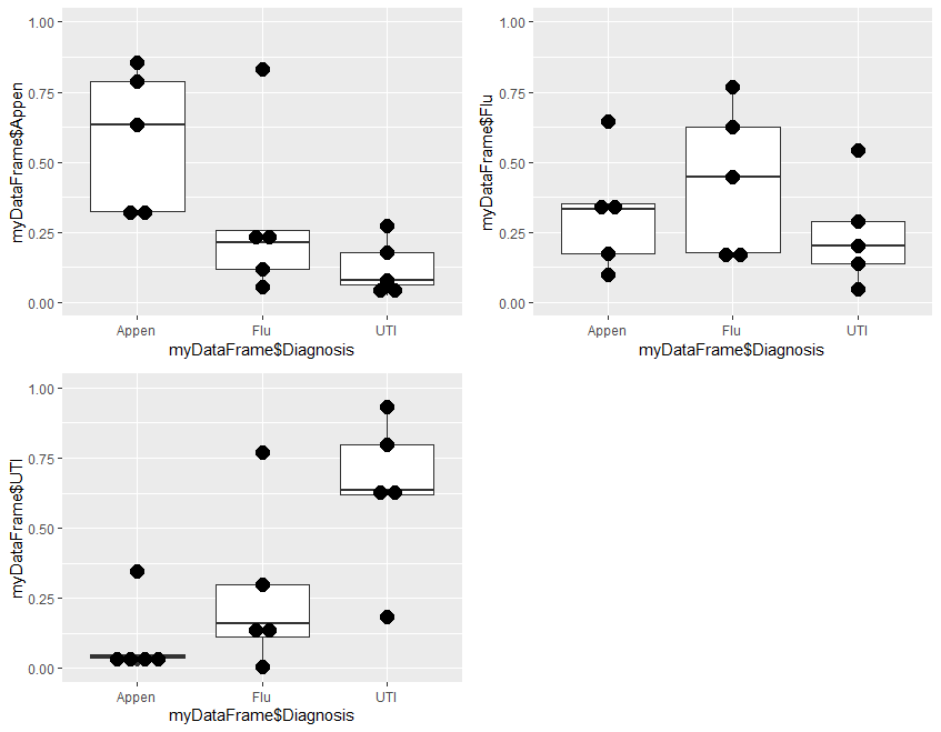Step 4 is optional, and plots the results to visually demonstrate the results of analysis. It is divided into two parts. Step 4a produces 3 plots, and step 4b combines these 3 plots into a single one for presentation # Step 4a: Plot 3 charts #install.packages("ggplot2") # if not already installed library(ggplot2) plot1<-ggplot(myDataFrame, aes(x = myDataFrame$Diagnosis, y = myDataFrame$Appen)) + coord_cartesian(ylim= c(0, 1)) + geom_boxplot() + geom_dotplot(binaxis="y",binwidth=.05,stackdir="center") #fitted Appen probability plot2<-ggplot(myDataFrame, aes(x = myDataFrame$Diagnosis, y = myDataFrame$UTI)) + coord_cartesian(ylim= c(0, 1)) + geom_boxplot() + geom_dotplot(binaxis="y",binwidth=.05,stackdir="center") #fitted Flu probability plot3<-ggplot(myDataFrame, aes(x = myDataFrame$Diagnosis, y = myDataFrame$Flu)) + coord_cartesian(ylim= c(0, 1)) + geom_boxplot() + geom_dotplot(binaxis="y",binwidth=.05,stackdir="center") #fitted UTI probability #Plot1 #plot2 #plot3 Plot1 plots the probability of Appen in the 3 groups of Appen, Flu, and UTI. Plot2 the probability of Flu and plot3 the probability of UTI in the same 3 groups. At this stage, the 3 plots can be separately displayed. The problem is that, in RStudio, each plot over-writes the previous one, so the 3 cannot be visualized at the same time. To do this, we need to do 4b. # Step 4b: Combine 3 charts into one #install.packages("Grid") # only if not already installed library(grid) # Make a list from the ... arguments and plotlist myPlots <- c(list(plot1, plot2, plot3)) #change list to your list of ggplots myCols = 2 #change the number of plot columns per row of plots # The rest of the codes need no change myNumPlots = length(myPlots) layout <- matrix(seq(1, myCols * ceiling(myNumPlots/myCols)), ncol = myCols, nrow = ceiling(myNumPlots/myCols)) grid.newpage() pushViewport(viewport(layout = grid.layout(nrow(layout), ncol(layout)))) # Make each plot, in the correct location for (i in 1:myNumPlots) { # Get the i,j matrix positions of the regions that contain this subplot matchidx <- as.data.frame(which(layout == i, arr.ind = TRUE)) print(myPlots[[i]], vp = viewport(layout.pos.row = matchidx$row, layout.pos.col = matchidx$col)) } In step 4b, the 3 plots are combined into a single one. It can be seen that, even though no statistical significance has been achieved, the probability estimates for Appen is highest in the Appen group in plot1, the probability estimates of FLU highest in the Flu group in plot2, and probability estimates of UTI highest in the UTI group in plot3. Step 5 is optional and for demonstration only. It shows how the results produced can be used to calculate and estimate the value for each case in a different dataset. Step 5a creates a new dataframe using the first 3 rows of the original data. Step 5b Predict with type='probs' produces the 3 columns of probability, and type='class' the classification. These can then be concatenated to the dataframe, and displayed. # Step 5a Use the coefficients on a new set of data newDat = (" Vomit Pulse Temp No 74 102 Yes 68 97 No 78 99 ") newDataFrame <- read.table(textConnection(newDat),header=TRUE) summary(newDataFrame) $ Step 5b: newProbs <- predict(mulLogRegResults, newdata=newDataFrame, type='probs') newProbs # probabilies newDiag <- predict(mulLogRegResults, newdata=newDataFrame, type='class') newDiag # diagnosis newDataFrame <- cbind(newDataFrame, newProbs, newDiag) # add to data frame newDataFrame The results are as follows > summary(newDataFrame) Vomit Pulse Temp No :2 Min. :68.00 Min. : 97.00 Yes:1 1st Qu.:71.00 1st Qu.: 98.00 Median :74.00 Median : 99.00 Mean :73.33 Mean : 99.33 3rd Qu.:76.00 3rd Qu.:100.50 Max. :78.00 Max. :102.00 > newProbs Appen Flu UTI 1 0.31691544 0.64513376 0.03795079 2 0.02178191 0.04675669 0.93146140 3 0.25714354 0.44566188 0.29719458 > newDiag [1] Flu UTI Flu Levels: Appen Flu UTI > > newDataFrame Vomit Pulse Temp Appen Flu UTI newDiag 1 No 74 102 0.31691544 0.64513376 0.03795079 Flu 2 Yes 68 97 0.02178191 0.04675669 0.93146140 UTI 3 No 78 99 0.25714354 0.44566188 0.29719458 Flu Please note the following The formula in step 3 cannot be use, as it requires that the dataframe has the same name and has the same number of rows as the original data. With the procedure in step 5a, a dataframe of different name and different number of rows can be handled. However, the names of the columns used for calculation must still be the same as that from the original dataframe. #Step 6: Optional saving and loading of coefficients #save(mulLogRegResults, file = "MulLogRegResults.rda") #save results to rda file #load("MulLogRegResults.rda") #load the rda file Step 6 is optional, and in fact commented out, and included as a template only. It allows the results of analysis to be stored as a .rda file, that can be reloaded on a different occasion and used on a different dataset. Please note the following R Studio read and write files using the default User/Document/ folder. The path needs to be reset if the user wishes to save and load files using a specific folder. Discussion in the file I/O panel of the R_Exp.php Once loaded, the conditions for analysis are the same as that in step 5b. Contents of C:42 Contents of D:43 Contents of E:44 GLM: Dependent Variable with Negative Binomial Distribution Explanation R Code C D E This panel provides explanations and example R codes for Negative Binomial Regression, where the dependent variable is a discrete positive integer with a negative binomial distribution. Negative Binomial distribution is the reverse of the binomial distribution. Instead of stating a proportion, the statement is the number of one group is counted before a stated number of the other group is found. In Negative Binomial Regression, the algorithm is to estimate the number of one group found (failure, negative, 0, false) before finding each case of the other group (success, positive, 1, true), mostly counts of events or number of units. An examples is, instead of stating that the caesarean section rate is 20%, the Negative Binomial statement is having 4 vaginal deliveries for each Caesarean Section seen. Negative Binomial distribution is less rigid in its distribution assumptions than Poisson distribution, it is often adapted to analyse any measurements of discrete positive value where the Poisson distribution cannot be assured. The model Negative Binomial regression in the example on this page uses the same data as that in the Poisson panel. The results, other than minor rounding differences, are almost identical to the analysis assuming Poisson distribution. Negative Binomial regression, similar to other Generalized Linear Models, is conceptually and procedurally simple and easy to understand. The contraint however is that the count in the modelling data must be a positive integer, a value >0. When the expected count is low however, the count in some of the reference data may be zero, and this distorts the model. The remedy for this problem is to include a Zero Inflated Model in the algorithm, and this is explained in the R code panel References https://en.wikipedia.org/wiki/Negative_binomial_distribution https://ncss-wpengine.netdna-ssl.com/wp-content/themes/ncss/pdf/Procedures/NCSS/Negative_Binomial_Regression.pdf https://stats.idre.ucla.edu/r/dae/negative-binomial-regression/ https://stats.idre.ucla.edu/r/dae/zinb/ The data is computer generated to demonstrate the computation methods. It perports to be from a study of workload in the labour ward, collected from a number of hospitals. Time is the time of the 3 shifts, AM for morning, PM for afternoon, and Night. Day is for day of the week, being Weekday or Weekend, BLY is the total number of births last year in thousands. The model is to make a estimate the number of births per shift (Births) from these 3 parameters, assuming that Births is a count and conforms to the Negative Binomial distribution Step 1 is to create the data frame # Step 1: Data entry myDat = (" Time Day BLY Births PM Wday 4.5 6 PM Wend 5.6 4 Night Wday 6.0 3 PM Wday 5.9 8 Night Wday 5.2 3 AM Wend 5.8 4 Night Wend 5.9 7 AM Wend 5.0 0 Night Wday 5.5 4 Night Wday 4.1 6 PM Wday 5.4 3 Night Wday 4.2 5 PM Wday 4.7 3 AM Wday 4.4 4 AM Wend 4.7 2 Night Wend 4.8 5 PM Wend 4.8 6 PM Wday 4.5 5 AM Wday 5.0 9 ") myDataFrame <- read.table(textConnection(myDat),header=TRUE) summary(myDataFrame) The summary of input data is as follows > summary(myDataFrame) Time Day BLY Births AM :5 Wday:12 Min. :4.100 Min. :0.000 Night:7 Wend: 7 1st Qu.:4.600 1st Qu.:3.000 PM :7 Median :5.000 Median :4.000 Mean :5.053 Mean :4.579 3rd Qu.:5.550 3rd Qu.:6.000 Max. :6.000 Max. 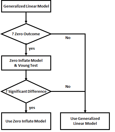:9.000 Strategy for Analysis The strategy of analysis is as shown in the flow chart to the left. The Generalized Linear Model (glm) for Negative Binomial distribution is used first, and if there is no zero values in the outcome, the analysis ends, and the results used If there is any zero outcome in the reference data, then the Zero Inflated Model (zi) is used, and the results compared with that from the glm model, using the Voung Test. Given that the two sets of analysis use the same data, the nested result is used. If the results from the glm and zi models are not significantly different, then the glm results are used. If there is a significant difference, then the zi results are used. The algorithm presented in this page provides analysis for both approaches, but this is redundant, as results from only one of the model should finally be presented Step 2 performs the Negaive Binomial analysis, and is divided into two parts. Step 2a uses the Generalized Linear Model (glm), 2b the Zero Inflated Model (zi), and 2c the comparison of the two to determine the results to be accepted Firstly step 2a, using the glm model. #Step 2: Negative Binomial Regression #Step 2a. using glm #install.packages(MASS) library(MASS) glmResults<-glm.nb(formula = Births ~ Time + Day + BLY, data = myDataFrame) glmCount<-fitted.values(glmResults) #count = exp(y) summary(glmResults) myDataFrame <- cbind(myDataFrame, glmCount) #append glmCount to myDataFrame myDataFrame The results are as follows glm.nb(formula = Births ~ Time + Day + BLY, data = myDataFrame, init.theta = 54599.73884, link = log) Deviance Residuals: Min 1Q Median 3Q Max -2.66322 -0.91210 -0.05635 0.47380 2.03454 Coefficients: Estimate Std. Error z value Pr(>|z|) (Intercept) 1.27840 0.92893 1.376 0.169 TimeNight 0.15967 0.30042 0.531 0.595 TimePM 0.21978 0.29647 0.741 0.458 DayWend -0.16692 0.24589 -0.679 0.497 BLY 0.03089 0.18594 0.166 0.868 (Dispersion parameter for Negative Binomial(54599.74) family taken to be 1) Null deviance: 21.614 on 18 degrees of freedom Residual deviance: 20.151 on 14 degrees of freedom AIC: 93.01 Number of Fisher Scoring iterations: 1 The results from Step 2a to focus on are the rows under the heading Estimate, as this is the formula for calculating the log(count). We will use the first row of data (Time=PM, Day=Wday, BLY=4.5) to demonstrate how this is done. We start with Y = Intercept = 1.27840 With Time=PM, Y = 1.27840 + 0.21978 With Day=Wday, Y = 1.27840 + 0.21978 + 0 With BLY=4.5, Y = 1.27840 + 0.21978 + 0 + 4.5(0.03089) Log(Countglm) = Y = 1.27840 + 0.21978 + 0 + 4.5(0.03089) = 1.637815 Countglm = exp(y) = exp(1.637815) = 5.140678116 There is however no need to manually calculate these values, as R does this as shown in step 2a. The last 3 lines of the code estimate Count using glm (glmCount), and append this to the dataframe Time Day BLY Births glmCount 1 PM Wday 4.5 6 5.140811 2 PM Wend 5.6 4 4.500898 3 Night Wday 6.0 3 5.070469 4 PM Wday 5.9 8 5.368042 5 Night Wday 5.2 3 4.946685 6 AM Wend 5.8 4 3.635224 7 Night Wend 5.9 7 4.277745 8 AM Wend 5.0 0 3.546479 9 Night Wday 5.5 4 4.992746 10 Night Wday 4.1 6 4.781402 11 PM Wday 5.4 3 5.285758 12 Night Wday 4.2 5 4.796196 13 PM Wday 4.7 3 5.172674 14 AM Wday 4.4 4 4.113756 15 AM Wend 4.7 2 3.513761 16 Night Wend 4.8 5 4.134812 17 PM Wend 4.8 6 4.391018 18 PM Wday 4.5 5 5.140811 19 AM Wday 5.0 9 4.190723 > Next, in step 2b performs the zero inflated analysis, produces the output count accordingly, and append the results to the data frame. The Vuong test compares the counts produced by the generalized linear model (glm) and zero inflated model (zi) and display whether the diffrence is significant. #install.packages("pscl") # only if not previously installed library(pscl) ziResults<-zeroinfl(Births ~ Time + Day + BLY, dist="negbin", data = myDataFrame) #zero inlation model summary(ziResults) ziCount <- predict(ziResults, myDataFrame) #zero inflated count myDataFrame <- cbind(myDataFrame,ziCount) #concatenate calculated count to myDataFrame myDataFrame The results are as follows zeroinfl(formula = Births ~ Time + Day + BLY, data = myDataFrame, dist = "negbin") Pearson residuals: Min 1Q Median 3Q Max -1.05117 -0.59996 -0.01863 0.49214 1.87321 Count model coefficients (negbin with log link): Estimate Std. Error z value Pr(>|z|) (Intercept) 1.51331 0.92356 1.639 0.101 TimeNight -0.01727 0.29613 -0.058 0.953 TimePM 0.04216 0.29228 0.144 0.885 DayWend -0.05730 0.24285 -0.236 0.813 BLY 0.01385 0.18458 0.075 0.940 Log(theta) 12.88701 167.64480 0.077 0.939 Zero-inflation model coefficients (binomial with logit link): Estimate Std. Error z value Pr(>|z|) (Intercept) -14.445 18942.295 -0.001 0.999 TimeNight -20.209 25664.897 -0.001 0.999 TimePM -20.310 25826.329 -0.001 0.999 DayWend 20.276 18942.290 0.001 0.999 BLY -1.281 3.020 -0.424 0.672 Theta = 395147.6678 Number of iterations in BFGS optimization: 24 Log-likelihood: -38.26 on 11 Df > ziCount <- predict(ziResults, myDataFrame) #zero inflated count > myDataFrame <- cbind(myDataFrame,ziCount) #concatenate calculated count to myDataFrame > myDataFrame Time Day BLY Births glmCount ziCount 1 PM Wday 4.5 6 5.140811 5.041842 2 PM Wend 5.6 4 4.500898 4.834124 3 Night Wday 6.0 3 5.070469 4.850651 4 PM Wday 5.9 8 5.368042 5.140529 5 Night Wday 5.2 3 4.946685 4.797217 6 AM Wend 5.8 4 3.635224 3.864226 7 Night Wend 5.9 7 4.277745 4.574173 8 AM Wend 5.0 0 3.546479 2.937645 9 Night Wday 5.5 4 4.992746 4.817185 10 Night Wday 4.1 6 4.781402 4.724706 11 PM Wday 5.4 3 5.285758 5.105064 12 Night Wday 4.2 5 4.796196 4.731252 13 PM Wday 4.7 3 5.172674 5.055823 14 AM Wday 4.4 4 4.113756 4.827030 15 AM Wend 4.7 2 3.513761 2.502474 16 Night Wend 4.8 5 4.134812 4.505033 17 PM Wend 4.8 6 4.391018 4.780872 18 PM Wday 4.5 5 5.140811 5.041842 19 AM Wday 5.0 9 4.190723 4.867299 Finally, in step 2c, the results from the Generalized Linear and Zero Inflated models are compared, using the Vuong Test. The Spearman's Correlation Coefficient is used for comparison vuong(glmResults, ziResults)# comparing the two models cor.test( ~ as.numeric(Births) + as.numeric(glmCount), data=myDataFrame, method = "spearman",exact=FALSE) cor.test( ~ as.numeric(Births) + as.numeric(ziCount), data=myDataFrame, method = "spearman",exact=FALSE) cor.test( ~ as.numeric(glmCount) + as.numeric(ziCount), data=myDataFrame, method = "spearman",exact=FALSE) The results are as follows > > vuong(glmResults, ziResults)# comparing the two models Vuong Non-Nested Hypothesis Test-Statistic: (test-statistic is asymptotically distributed N(0,1) under the null that the models are indistinguishible) ------------------------------------------------------------- Vuong z-statistic H_A p-value Raw -0.7669298 model2 > model1 0.22156 AIC-corrected 0.9437815 model1 > model2 0.17264 BIC-corrected 1.7516127 model1 > model2 0.03992 > Spearman's rank correlation rho > cor.test( ~ as.numeric(Births) + as.numeric(glmCount), data=myDataFrame, method = "spearman",exact=FALSE) S = 976.91, p-value = 0.559, rho = 0.1430578 > cor.test( ~ as.numeric(Births) + as.numeric(ziCount), data=myDataFrame, method = "spearman",exact=FALSE) S = 896.89, p-value = 0.3807 rho = 0.2132539 > cor.test( ~ as.numeric(glmCount) + as.numeric(ziCount), data=myDataFrame, method = "spearman",exact=FALSE) data: as.numeric(glmCount) and as.numeric(ziCount) S = 178.16, p-value = 5.647e-06, rho = 0.8437226 The results of the zero inflated analysis presents coefficients for combined Negative Binomial and Binmomial distributions to be used in estimating the counts. The method of calculation using these coefficients is by numerical approximation, and too complex to be explained here. Those interested in numerical methods should consult the references provided. 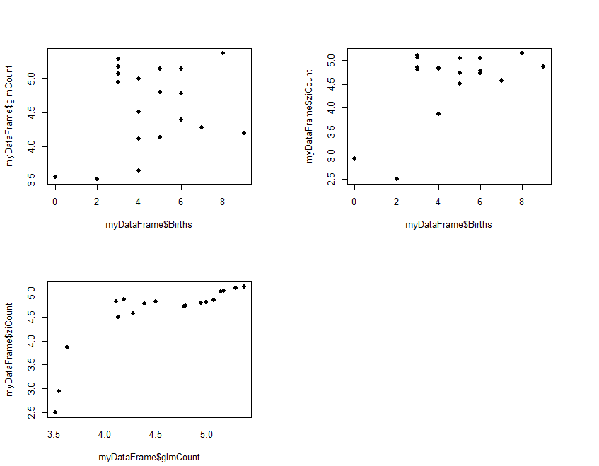The results (ziCount) are then compared with those from the generalized linear model (glmCount) using the Voung test. The test produced by the basic calculation is labelled Raw, AIC has a correction by Akaike's information criterion, and BIC has a correction by the Bayesian information criterion. In practice they are different methods of calculating the same thing. One way of interpreting the 3 results is to assume that the two models are different if any of the 3 comparisons is statistically significant, as is the case with the current example data. The 3 Spearman's correlations test how closely the two estimates related to the original outcome, and to each other. The results shows that both performed poorly with the reference outcome (Births:glmCount, ρ=0.14; Births:ziCount, ρ=0.21; both not statistically significant). The two estimates however are closely but not perfectly correlated to each other (glmCount:ziCount, ρ=0.84, p<0.0001). Such poor results are not surprising, given that the data is randomly generated by the computer and the sample size very small. It merely serves to demonstrate the numerical methods. Step 3 is optional and plots the fitted values #Step 3: Plot fitted values old.par <- par(mfrow=c(2,2)) par(pin=c(3, 2)) # set plotting window to 4.2x3 inches plot(x = myDataFrame$Births, # Births on the x axis y = myDataFrame$glmCount, # glmCount on the y axis xlim = c(min(myDataFrame$Births),max(myDataFrame$Births)), ylim = c(min(myDataFrame$glmCount),max(myDataFrame$glmCount)), pch = 16) # size of dot plot(x = myDataFrame$Births, # Births on the x axis y = myDataFrame$ziCount, # ziCount on the y axis xlim = c(min(myDataFrame$Births),max(myDataFrame$Births)), ylim = c(min(myDataFrame$ziCount),max(myDataFrame$ziCount)), pch = 16) # size of dot plot(x = myDataFrame$glmCount, # Births on the x axis y = myDataFrame$ziCount, # ziCount on the y axis xlim = c(min(myDataFrame$glmCount),max(myDataFrame$glmCount)), ylim = c(min(myDataFrame$ziCount),max(myDataFrame$ziCount)), pch = 16) # size of dot par(old.par) Step 3 produces 3 plots in the same view, each a scatterplot for a pair in the 3 counts of Births, glmCont, and ziCount. The plot is optional, but allows the analyst to examine and compare the different results. Step 4 is optional and for demonstration only. It shows how the results produced can be used to calculate and estimate the value for each case in a different dataset. Step 4a creates a new dataframe using the first 3 rows of the original data. Step 4b Predict with type='response' to produce both the glmCount and ziCount. These can then be concatenated to the dataframe, and displayed. # Step 4a: Test coefficients on new data set newDat = (" Time Day BLY PM Wday 4.5 Night Wday 6.0 AM Wend 5.8 ") newDataFrame <- read.table(textConnection(newDat),header=TRUE) summary(newDataFrame) # Step 4b: Calculate results using new data newGlmCount <- predict(glmResults, newdata=newDataFrame, type='response') newZiCount <- predict(ziResults, newdata=newDataFrame, type='response') newDataFrame <- cbind(newDataFrame, newGlmCount, newZiCount) newDataFrame The results are as follows. Please note that, in practice, only one of the counts need to be estimated, as by this stage a decision whether glm or zi should be used has been made. The results are presented as follows Time Day BLY newGlmCount newZiCount 1 PM Wday 4.5 5.140811 5.041842 2 Night Wday 6.0 5.070469 4.850651 3 AM Wend 5.8 3.635224 3.864226 Please note the following The formula in step 2 cannot be use, as it requires that the dataframe has the same name and has the same number of rows as the original data. With the procedure in step 4, a dataframe of different name and different number of rows can be handled. However, the names of the columns used for calculation must still be the same as that from the original dataframe. Step 5 is optional, the saving of the coefficients, and loading them is future use #Step 5: Optional saving and loading of coefficients #save(glmResults, file = "NegBinGlmResults.rda") #save glm results to rda file #load("NegBinGlmResults.rda") #load the glm rda file #save(ziResults, file = "NegBinZiResults.rda") #save zi results to rda file #load("NegBinZiResults.rda") #load the zi rda file Please note that the codes are commented out as they are optional, and included as a template only. It allows the results of analysis to be stored as a .rda file, that can be reloaded on a different occasion and used on a different dataset. Please note the following R Studio read and write files using the default User/Document/ folder. The path needs to be reset if the user wishes to save and load files using a specific folder. Discussion in the file I/O panel of the R_Exp.php Once loaded, the conditions for analysis are the same as that in step 4. Contents of C:52 Contents of D:53 Contents of E:54 GLM: Dependent Variable with Ordinal Distribution Explanation R Code C D E This panel provides explanations and example R codes for Ordinal Logistic Regression, which is one of the algorithms based on the Generalized Linear Models. Ordinal Regression is a variant of the Multinomial Regression model, as explained in the previous panel, but the dependent variable is ordinal, in that they are ordered in scale alphabetically, so the grp1<Grp2<Grp3 ... In R, the independent variables can be measurements or factors Measurements are numerical, and can be binary(0/1), ordinal, or parametric Factors are text, and consists of group names. Unless otherwise assigned, R arrange group names alphabetically, and use the first name as the reference group The algorithm produces m-1 formulae, m being the number of groups. The probabilities of belonging to the groups are estimated, and the estimated diagnosis assigned to that with the highest probability. Details on how this is carried out are described in the R code panel References https://en.wikipedia.org/wiki/Ordered_logit https://stats.idre.ucla.edu/r/dae/ordinal-logistic-regression/ The data presented here are computer generated. It purports to be from a study on factors that predicts the success of breast feeding. The predictors are whether they received antenatal breast feeding counselling (Counsel = No/Yes), level of education (Educ = Primary/Secondary/Tertiary), and age in completed years (Age). Outcomes are level success in breast feeding with the following levels (BFeed) S0 = not breast feeding al all S1 = Breast feeding successfully at time of leaving hospital S2 = Breast feeding still 1 month after birth S3 = Breast feeding still 6 months after birth There are 13 cases (rows in the data Step 1: Creates the data frame for analysis # Step 1: Data entry to dataframe myDat = (" # Step 1: Data entry myDat = (" Counsel Educ Age BFeed No Tertiary 27 S3 No Tertiary 29 S1 Yes Secondary 27 S1 No Primary 37 S2 No Tertiary 27 S0 No Primary 37 S3 Yes Secondary 25 S0 Yes Primary 33 S1 No Tertiary 35 S2 Yes Secondary 29 S1 No Primary 25 S0 Yes Tertiary 33 S2 Yes Secondary 27 S3 ") myDataFrame <- read.table(textConnection(myDat),header=TRUE) summary(myDataFrame) The summary of the data is as follows > summary(myDataFrame) Counsel Educ Age BFeed No :7 Primary :4 Min. :25.00 S0:3 Yes:6 Secondary:4 1st Qu.:27.00 S1:4 Tertiary :5 Median :29.00 S2:3 Mean :30.08 S3:3 3rd Qu.:33.00 Max. :37.00 Step 2: Ordinal Regression # Step 2: Ordinal Regression #install.packages("MASS") # if not already installed library(MASS) ordRegResults <- polr(BFeed ~ Counsel + Educ + Age, data = myDataFrame, Hess=TRUE) summary(ordRegResults) The results are as follows Call: polr(formula = BFeed ~ Counsel + Educ + Age, data = myDataFrame, Hess = TRUE) Coefficients: Value Std. Error t value CounselYes -0.353 1.340 -0.263 EducSecondary 2.319 2.122 1.093 EducTertiary 1.229 1.371 0.896 Age 0.427 0.206 2.073 Intercepts: Value Std. Error t value S0|S1 12.36 6.75 1.83 S1|S2 14.52 7.19 2.02 S2|S3 15.87 7.35 2.16 Residual Deviance: 29.90 AIC: 43.90 The results from Step 2 to focus on are the rows under the heading Value in the two sets of Coefficients and Intercepts. We will use the first row of the data as an example of calculation (Counsel=No, Educ=Tertiary, Age=27) The probabilities of each level are calculated as follows For S0 To start, YS0 = Intercept(S0|S1) = 12.36 Counsel=No, YS0 = 12.36 - (0) Educ=Tertiary, YS0 = 12.36 - (0 + 1.229) Age=27, YS0 = 12.36 - (0 + 1.229 + 27(0.427)) LogitS0 = YS0 = 12.36 - (0 + 1.229 + 27(0.427)) = -0.398 Probability PS0 = 1 / (1 + exp(-LogitS0)) = 1 / (1+exp(0.398)) = 0.40 For S1, the formula is the same except for the Intercept (S1|S2) = 14.52 LogitS1 = YS1 = 14.52 - (0 + 1.229 + 27(0.427)) = 1.762 Uncorrected Probability UPS1 = 1 / (1 + exp(-LogitS1)) = 1 / (1+exp(-1.762)) = 0.85 The corrected Probability PS1 = UPS1 - PS0 = 0.85 - 0.40 = 0.45 For S2, the formula is the same except for the Intercept (S2|S3) = 15.87 LogitS2 = YS2 = 15.87 - (0 + 1.229 + 27(0.427)) = 3.112 Uncorrected Probability UPS2 = 1 / (1 + exp(-LogitS2)) = 1 / (1+exp(-3.112)) = 0.96 The corrected Probability PS2 = UPS2 - UPS1 = 0.96 - 0.85 = 0.11 For the last group, S3, the probability PS3 = 1 - UPS2 = 1 - 0.96 = 0.04 There is however no need to manually calculate these values, as R does this as shown in step 3. In step 3a, the fitted.values function creates the 4 columns of probabilities for the levels of outcomes, and the predict function make the decision which outcome is the most likely. The cbind function concatenates these results to the dataframe, which is then displayed. Step 3b creates the 4x4 table of counts between the original Diagnosis and the estimated myPredict, to test the accuracy of the algorithm. The Spearman's Correlation Coefficient estimates the precision of the prediction (0=random, 1=perfect). # Step 3a: Place fitted values into data frame and display results myFitted<-round(fitted.values(ordRegResults),4) myPredict <- predict(ordRegResults, myDataFrame) myDataFrame <- cbind(myDataFrame, myFitted, myPredict) myDataFrame #optional display of data frame The results are as follows Counsel Educ Age BFeed S0 S1 S2 S3 myPredict 1 No Tertiary 27 S3 0.4049 0.4502 0.1027 0.0423 S1 2 No Tertiary 29 S1 0.2247 0.4906 0.1908 0.0939 S1 3 Yes Secondary 27 S1 0.2455 0.4928 0.1772 0.0845 S1 4 No Primary 37 S2 0.0316 0.1889 0.3003 0.4792 S3 5 No Tertiary 27 S0 0.4049 0.4502 0.1027 0.0423 S1 6 No Primary 37 S3 0.0316 0.1889 0.3003 0.4792 S3 7 Yes Secondary 25 S0 0.4331 0.4357 0.0934 0.0378 S1 8 Yes Primary 33 S1 0.2037 0.4855 0.2058 0.1051 S1 9 No Tertiary 35 S2 0.0219 0.1408 0.2647 0.5726 S3 10 Yes Secondary 29 S1 0.1218 0.4241 0.2761 0.1780 S1 11 No Primary 25 S0 0.8451 0.1342 0.0152 0.0055 S0 12 Yes Tertiary 33 S2 0.0696 0.3239 0.3202 0.2863 S1 13 Yes Secondary 27 S3 0.2455 0.4928 0.1772 0.0845 S1 # Step 3b with(myDataFrame, table(BFeed,myPredict)) #check table of prediction cor.test( ~ as.numeric(BFeed) + as.numeric(myPredict), data=myDataFrame, method = "spearman",exact=FALSE) The results are > with(myDataFrame, table(BFeed,myPredict)) #check table of prediction myPredict BFeed S0 S1 S2 S3 S0 1 2 0 0 S1 0 4 0 0 S2 0 1 0 2 S3 0 2 0 1 > cor.test( ~ as.numeric(BFeed) + as.numeric(myPredict), data=myDataFrame, method = "spearman",exact=FALSE) Spearman's rank correlation rho S = 200, p-value = 0.05, rho = 0.55 The dataframe now contains the original columns, plus the 4 columns of probability for each level of outcome, as well as the conclusion which level is most likely. The table shows the correct prediction along the diagonal, 6 cases out of 13. 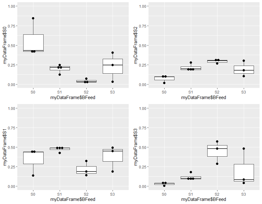The Spearman's correlation coefficient is 0.55 Step 4 is optional, and plots the results to visually demonstrate the results of analysis. It is divided into two parts. Step 4a produces 4 plots, and step 4b combines these 4 plots into a single one for presentation #Step 4a: Make 4 different plots #install.packages("ggplot2") # if not already installed library(ggplot2) plot1<-ggplot(myDataFrame, aes(x = myDataFrame$BFeed, y = myDataFrame$S0)) + coord_cartesian(ylim= c(0, 1)) + geom_boxplot() + geom_dotplot(binaxis="y",binwidth=.03, stackdir="center") plot2<-ggplot(myDataFrame, aes(x = myDataFrame$BFeed, y = myDataFrame$S1, ymin=0.0, ymax=1.0)) + coord_cartesian(ylim= c(0, 1)) + geom_boxplot() + geom_dotplot(binaxis="y",binwidth=.03, stackdir="center") plot3<-ggplot(myDataFrame, aes(x = myDataFrame$BFeed, y = myDataFrame$S2, ymin=0.0, ymax=1.0)) + coord_cartesian(ylim= c(0, 1)) + geom_boxplot() + geom_dotplot(binaxis="y",binwidth=.03, stackdir="center") plot4<-ggplot(myDataFrame, aes(x = myDataFrame$BFeed, y = myDataFrame$S3, ymin=0.0, ymax=1.0)) + coord_cartesian(ylim= c(0, 1)) + geom_boxplot() + geom_dotplot(binaxis="y",binwidth=.03, stackdir="center") #plot1 #plot2 #plot3 #plot4 Plot1 plots the estimated probability of S0 for the 4 levels of outcome in the original data, plot2 the probability of S1, plot3 the probability of S2, and plot4 the probability of S3. At this stage, the 4 plots can be separately displayed. The problem is that, in RStudio, each plot over-writes the previous one, so the 4 cannot be visualized at the same time. To do this, we need to do step 4b. # Step 4b: Combine 4 plots into 1 #install.packages("Grid") # if not already installed library(grid) # Make a list from the ... arguments and plotlist myPlots <- c(list(plot1,plot2,plot3,plot4)) #change list to your list of ggplots myCols = 2 #change the number of plot columns per row of plots # The rest of the codes need no change myNumPlots = length(myPlots) layout <- matrix(seq(1, myCols * ceiling(myNumPlots/myCols)), ncol = myCols, nrow = ceiling(myNumPlots/myCols)) grid.newpage() pushViewport(viewport(layout = grid.layout(nrow(layout), ncol(layout)))) # Make each plot, in the correct location for (i in 1:myNumPlots) { # Get the i,j matrix positions of the regions that contain this subplot matchidx <- as.data.frame(which(layout == i, arr.ind = TRUE)) print(myPlots[[i]], vp = viewport(layout.pos.row = matchidx$row, layout.pos.col = matchidx$col)) } In step 4b, the 4 plots are combined into a single one. It can be seen that, even though no statistical significance has been achieved, the probability estimates for S0 is highest for the S0 level, probability of S1 the highest for S1 level, and probability of S2 highest for the S2 level. However, S3 is poorly estimated. These suboptimal results are not surprising given that the data is computer generated random values, and the sample size is very small. Step 5 is optional and for demonstration only. It shows how the results produced can be used to calculate and estimate the value for each case in a different dataset. Step 5a creates a new dataframe with 4 rows of data. Step 5b predicts with type='probs' produces the 3 columns of probability, and type='class' the classification. These can then be concatenated to the dataframe, and displayed. # Step 5a: Creates a different set of data newDat = (" Counsel Educ Age No Tertiary 27 No Tertiary 29 Yes Secondary 25 Yes Tertiary 33 ") newDataFrame <- read.table(textConnection(newDat),header=TRUE) summary(newDataFrame) #step 5b: Test coefficients on new set of data newProbs <- predict(ordRegResults, newdata=newDataFrame, type='probs') newProbs newDiag <- predict(ordRegResults, newdata=newDataFrame, type='class') newDiag # Add results to new data frame newDataFrame <- cbind(newDataFrame, newProbs, newDiag) newDataFrame The results are shown as follows Counsel Educ Age S0 S1 S2 S3 newDiag 1 No Tertiary 27 0.40 0.45 0.103 0.042 S1 2 No Tertiary 29 0.22 0.49 0.191 0.094 S1 3 Yes Secondary 25 0.43 0.44 0.093 0.038 S1 4 Yes Tertiary 33 0.07 0.32 0.320 0.286 S1 Please note the following The formula in step 3 cannot be use, as it requires that the dataframe has the same name and has the same number of rows as the original data. With the procedure in step 5, a dataframe of different name and different number of rows can be handled. However, the names of the columns used for calculation must still be the same as that from the original dataframe. Step 6 is optional, saving th coefficients for future use #Step 6: Optional saving and loading of coefficients #save(ordRegResults, file = "OrdRegResults.rda") #save results to rda file #load("OrdRegResults.rda") #load the rda file Step 6 is optional, and in fact commented out, and included as a template only. It allows the results of analysis to be stored as a .rda file, that can be reloaded on a different occasion and used on a different dataset. Please note the following R Studio read and write files using the default User/Document/ folder. The path needs to be reset if the user wishes to save and load files using a specific folder. Discussion in the file I/O panel of the R_Exp.php Once loaded, the conditions for analysis are the same as that in step 5. Contents of C:62 Contents of D:63 Contents of E:64 GLM: Dependent Variable with Poisson Distribution (Counts) Explanation R Code C D E This page provides explanations and example R codes for Poisson Regression, where the dependent variable is a discrete positive integer with Poisson distribution, mostly counts of events or number of units in a defined environment. Examples are the number of cells seen in a field under the microscope, the number of asthma attacks per 100 child year, the number of pregnancies per 100 women year using a particular form of contraception. The Poisson Regression is a powerful analytical tool, providing that the data conforms to the Poisson distribution. When there is doubt about the distribution, the less powerful methods with less rigorous assumptions should be used. These are the Ordinal Regression or the Negative Binomial Regression, as explained in the other panels of this page Poisson regression, similar to other Generalized Linear Models, is conceptually and procedurally simple and easy to understand. The contraint however is that the count in the modelling data must be a positive integer, a value >0. When the expected count is low however, the count in some of the reference data may be zero, and this distorts the model. The remedy for this problem is to include a Zero Inflated Model in the algorithm, and this is explained in the R code panel References https://en.wikipedia.org/wiki/Poisson_regression https://stats.idre.ucla.edu/r/dae/poisson-regression/ https://stats.idre.ucla.edu/r/dae/zip/ https://en.wikipedia.org/wiki/Zero-inflated_model https://en.wikipedia.org/wiki/Vuong%27s_closeness_test https://www.rdocumentation.org/packages/mpath/versions/0.1-20/topics/vuong.test The data is computer generated to demonstrate the computation methods. It perports to be from a study of workload in the labour ward, collected from a number of hospitals. Time is the time of the 3 shifts, AM for morning, PM for afternoon, and Night. Day is for day of the week, being Weekday or Weekend, BLY is the total number of births last year in thousands. The model is to make a estimate the number of births per shift (Births) from these 3 parameters, assuming that Births is a count and conforms to the Poisson distribution Step 1 creates the dataframe that contains the data as in myDat. # Step 1: Data entry myDat = (" Time Day BLY Births PM Wday 4.5 6 PM Wend 5.6 4 Night Wday 6.0 3 PM Wday 5.9 8 Night Wday 5.2 3 AM Wend 5.8 4 Night Wend 5.9 7 AM Wend 5.0 0 Night Wday 5.5 4 Night Wday 4.1 6 PM Wday 5.4 3 Night Wday 4.2 5 PM Wday 4.7 3 AM Wday 4.4 4 AM Wend 4.7 2 Night Wend 4.8 5 PM Wend 4.8 6 PM Wday 4.5 5 AM Wday 5.0 9 ") myDataFrame <- read.table(textConnection(myDat),header=TRUE) summary(myDataFrame) The summary of the input data is as follows > summary(myDataFrame) Time Day BLY Births AM :5 Wday:12 Min. :4.100 Min. :0.000 Night:7 Wend: 7 1st Qu.:4.600 1st Qu.:3.000 PM :7 Median :5.000 Median :4.000 Mean :5.053 Mean :4.579 3rd Qu.:5.550 3rd Qu.:6.000 Max. :6.000 Max. :9.000 Strategy for Analysis The strategy of analysis is as shown in the flow chart to the left. The Generalized Linear Model (glm) for Poisson distribution is used first, and if there is no zero values in the outcome, the analysis ends, and the results used If there is any zero outcome in the reference data, then the Zero Inflated Model (zi) is used, and the results compared with that from the glm model, using the Voung Test. Given that the two sets of analysis use the same data, the nested result is used. If the results from the glm and zi models are not significantly different, then the glm results are used. If there is a significant difference, then the zi results are used. The algorithm presented in this page provides analysis for both approaches, but this is redundant, as results from only one of the model should finally be presented Step 2 performs the Poisson analysis, and is divided into two parts. Step 2a uses the Generalized Linear Model (glm), and 2b the Zero Inflated Model (zi) Step 2a performs the analysis using the glm model. The results are as follows #Step 2a. using glm glmResults<-glm(formula = Births ~ Time + Day + BLY, data = myDataFrame, family=poisson()) summary(glmResults) #display results glmCount<-fitted.values(glmResults) #count = exp(y) myDataFrame <- cbind(myDataFrame, glmCount) #append glmCount to myDataFrame myDataFrame The results are as follows Call: glm(formula = Births ~ Time + Day + BLY, family = poisson(), data = myDataFrame) Deviance Residuals: Min 1Q Median 3Q Max -2.66327 -0.91213 -0.05635 0.47382 2.03464 Coefficients: Estimate Std. Error z value Pr(>|z|) (Intercept) 1.27841 0.92889 1.376 0.169 TimeNight 0.15966 0.30041 0.531 0.595 TimePM 0.21978 0.29646 0.741 0.458 DayWend -0.16691 0.24588 -0.679 0.497 BLY 0.03089 0.18593 0.166 0.868 (Dispersion parameter for poisson family taken to be 1) Null deviance: 21.615 on 18 degrees of freedom Residual deviance: 20.153 on 14 degrees of freedom AIC: 91.01 Number of Fisher Scoring iterations: 5 The results from Step 2a to focus on are the rows under the heading Estimate, as this is the formula for calculating the log(count). We will use the first row of data (Time=PM, Day=Wday, BLY=4.5) to demonstrate how this is done. We start with Y = Intercept = 1.27841 With Time=PM, Y = 1.27841 + 0.21978 With Day=Wday, Y = 1.27841 + 0.21978 + 0 With BLY=4.5, Y = 1.27841 + 0.21978 + 0 + 4.5(0.03089) Log(Countglm) = Y = 1.27841 + 0.21978 + 0 + 4.5(0.03089) = 1.637195 Countglm = exp(y) = exp(1.637195) = 5.140729523 There is however no need to manually calculate these values, as R does this as shown in step 2a. The last 3 lines of the code estimate Count using glm (glmCount), and append this to the dataframe Time Day BLY Births glmCount 1 PM Wday 4.5 6 5.140809 2 PM Wend 5.6 4 4.500904 3 Night Wday 6.0 3 5.070451 4 PM Wday 5.9 8 5.368030 5 Night Wday 5.2 3 4.946672 6 AM Wend 5.8 4 3.635237 7 Night Wend 5.9 7 4.277743 8 AM Wend 5.0 0 3.546494 9 Night Wday 5.5 4 4.992731 10 Night Wday 4.1 6 4.781396 11 PM Wday 5.4 3 5.285749 12 Night Wday 4.2 5 4.796190 13 PM Wday 4.7 3 5.172670 14 AM Wday 4.4 4 4.113764 15 AM Wend 4.7 2 3.513777 16 Night Wend 4.8 5 4.134816 17 PM Wend 4.8 6 4.391029 18 PM Wday 4.5 5 5.140809 19 AM Wday 5.0 9 4.190728 Next, step 2b calculates the Zero-inflation, and adds the results to the data frame #Step 2b. Zero-inflation #install.packages("pscl") # only if not previously installed library(pscl) ziResults<-zeroinfl(Births ~ Time + Day + BLY, dist="poisson", data = myDataFrame) #zero inlation model summary(ziResults) ziCount <- predict(ziResults, myDataFrame) #zero inflated count myDataFrame <- cbind(myDataFrame,ziCount) #concatenate calculated count to myDataFrame The results are as follows zeroinfl(formula = Births ~ Time + Day + BLY, data = myDataFrame, dist = "poisson") Pearson residuals: Min 1Q Median 3Q Max -1.05159 -0.59996 -0.01862 0.49214 1.87321 Count model coefficients (poisson with log link): Estimate Std. Error z value Pr(>|z|) (Intercept) 1.51333 0.92356 1.639 0.101 TimeNight -0.01729 0.29613 -0.058 0.953 TimePM 0.04214 0.29228 0.144 0.885 DayWend -0.05728 0.24285 -0.236 0.814 BLY 0.01384 0.18458 0.075 0.940 Zero-inflation model coefficients (binomial with logit link): Estimate Std. Error z value Pr(>|z|) (Intercept) -14.472 18736.205 -0.001 0.999 TimeNight -20.209 25675.676 -0.001 0.999 TimePM -20.310 25837.885 -0.001 0.999 DayWend 20.249 18736.200 0.001 0.999 BLY -1.270 3.015 -0.421 0.674 Number of iterations in BFGS optimization: 17 Log-likelihood: -38.26 on 10 Df > ziCount <- predict(ziResults, myDataFrame) #zero inflated count > myDataFrame <- cbind(myDataFrame,ziCount) #concatenate calculated count to myDataFrame > myDataFrame Time Day BLY Births glmCount ziCount 1 PM Wday 4.5 6 5.140809 5.041806 2 PM Wend 5.6 4 4.500904 4.834177 3 Night Wday 6.0 3 5.070451 4.850580 4 PM Wday 5.9 8 5.368030 5.140475 5 Night Wday 5.2 3 4.946672 4.797157 6 AM Wend 5.8 4 3.635237 3.859393 7 Night Wend 5.9 7 4.277743 4.574203 8 AM Wend 5.0 0 3.546494 2.938806 9 Night Wday 5.5 4 4.992731 4.817121 10 Night Wday 4.1 6 4.781396 4.724659 11 PM Wday 5.4 3 5.285749 5.105017 12 Night Wday 4.2 5 4.796190 4.731204 13 PM Wday 4.7 3 5.172670 5.055785 14 AM Wday 4.4 4 4.113764 4.827064 15 AM Wend 4.7 2 3.513777 2.507346 16 Night Wend 4.8 5 4.134816 4.505074 17 PM Wend 4.8 6 4.391029 4.780934 18 PM Wday 4.5 5 5.140809 5.041806 19 AM Wday 5.0 9 4.190728 4.867325 Finally, in step 2c, the results from the Generalized Linear and Zero Inflated models are compared, using the Vuong Test. The Spearman's Correlation Coefficient is used for comparison # Step 2c: Comparison of models vuong(glmResults, ziResults)# comparing the two models cor.test( ~ as.numeric(Births) + as.numeric(glmCount), data=myDataFrame, method = "spearman",exact=FALSE) cor.test( ~ as.numeric(Births) + as.numeric(ziCount), data=myDataFrame, method = "spearman",exact=FALSE) cor.test( ~ as.numeric(glmCount) + as.numeric(ziCount), data=myDataFrame, method = "spearman",exact=FALSE) The results are as follows > vuong(glmResults, ziResults)# comparing the two models Vuong Non-Nested Hypothesis Test-Statistic: (test-statistic is asymptotically distributed N(0,1) under the null that the models are indistinguishible) ------------------------------------------------------------- Vuong z-statistic H_A p-value Raw -0.7671979 model2 > model1 0.221482 AIC-corrected 0.9441481 model1 > model2 0.172547 BIC-corrected 1.7522791 model1 > model2 0.039863 > > cor.test( ~ as.numeric(Births) + as.numeric(glmCount), data=myDataFrame, method = "spearman",exact=FALSE) Spearman's rank correlation rho data: as.numeric(Births) and as.numeric(glmCount) S = 976.91, p-value = 0.559, rho = 0.1430578 > cor.test( ~ as.numeric(Births) + as.numeric(ziCount), data=myDataFrame, method = "spearman",exact=FALSE) S = 896.89, p-value = 0.3807, rho = 0.2132539 > cor.test( ~ as.numeric(glmCount) + as.numeric(ziCount), data=myDataFrame, method = "spearman",exact=FALSE) S = 178.16, p-value = 5.647e-06, rho = 0.8437226 The results of the zero inflated analysis presents coefficients for combined Poisson and Binmomial distributions to be used in estimating the counts. The method of calculation using these coefficients is by numerical approximation, and too complex to be explained here. Those interested in numerical methods should consult the references provided. The results (ziCount) are then compared with those from the generalized linear model (glmCount) using the Voung test. The test produced by the basic calculation is labelled Raw, AIC has a correction by Akaike's information criterion, and BIC has a correction by the Bayesian information criterion. In practice they are different methods of calculating the same thing. One way of interpreting the 3 results is to assume that the two models are different if any of the 3 comparisons is statistically significant, as is the case with the current example data. The 3 Spearman's correlations test how closely the two estimates related to the original outcome, and to each other. The results shows that both performed poorly with the reference outcome (Births:glmCount, ρ=0.14; Births:ziCount, ρ=0.21; both not statistically significant). The two estimates however are closely but not perfectly correlated to each other (glmCount:ziCount, ρ=0.84, p<0.0001). Such poor results are not surprising, given that the data is randomly generated by the computer and the sample size very small. It merely serves to demonstrate the numerical methods. Step 3 produces 3 plots in the same view, each a scatterplot for a pair in the 3 counts of Births, glmCont, and ziCount. The plot is optional, but allows the analyst to examine and compare the different results. #Step 3: Plot fitted values old.par <- par(mfrow=c(2,2)) par(pin=c(3, 2)) # set plotting window to 4.2x3 inches plot(x = myDataFrame$Births, # Births on the x axis y = myDataFrame$glmCount, # glmCount on the y axis xlim = c(min(myDataFrame$Births),max(myDataFrame$Births)), ylim = c(min(myDataFrame$glmCount),max(myDataFrame$glmCount)), pch = 16) # size of dot plot(x = myDataFrame$Births, # Births on the x axis y = myDataFrame$ziCount, # ziCount on the y axis xlim = c(min(myDataFrame$Births),max(myDataFrame$Births)), ylim = c(min(myDataFrame$ziCount),max(myDataFrame$ziCount)), pch = 16) # size of dot plot(x = myDataFrame$glmCount, # Births on the x axis y = myDataFrame$ziCount, # ziCount on the y axis xlim = c(min(myDataFrame$glmCount),max(myDataFrame$glmCount)), ylim = c(min(myDataFrame$ziCount),max(myDataFrame$ziCount)), pch = 16) # size of dot par(old.par) Step 3 produces 3 plots in the same view, each a scatterplot for a pair in the 3 counts of Births, glmCont, and ziCount. The plot is optional, but allows the analyst to examine and compare the different results. Step 4 is optional and for demonstration only. It shows how the results produced can be used to calculate and estimate the value for each case in a different dataset. Step 4 creates a new dataframe using the first 3 rows of the original data. Predict with type='response' to produce both the glmCount and ziCount. These can then be concatenated to the dataframe, and displayed. Please note that, in practice, only one of the counts need to be estimated, as by this stage a decision whether glm or zi should be used has been made. The results are presented as follows # Step 4: Test coefficients on new data set newDat = (" Time Day BLY PM Wday 4.5 Night Wday 6.0 AM Wend 5.8 ") newDataFrame <- read.table(textConnection(newDat),header=TRUE) summary(newDataFrame) newGlmCount <- predict(glmResults, newdata=newDataFrame, type='response') newZiCount <- predict(ziResults, newdata=newDataFrame, type='response') newDataFrame <- cbind(newDataFrame, newGlmCount, newZiCount) newDataFrame The results are as follows Time Day BLY newGlmCount newZiCount 1 PM Wday 4.5 5.140809 5.041806 2 Night Wday 6.0 5.070451 4.850580 3 AM Wend 5.8 3.635237 3.859393 Please note the following The formula in step 2 cannot be use, as it requires that the dataframe has the same name and has the same number of rows as the original data. With the procedure in step 4, a dataframe of different name and different number of rows can be handled. However, the names of the columns used for calculation must still be the same as that from the original dataframe. Step 5 is optional and demonstrates saving the coefficients in a file and loading them in future use #Step 5: Optional saving and loading of coefficients #save(glmResults, file = "PoissonGlmResults.rda") #save glm results to rda file #load("PoissonGlmResults.rda") #load the glm rda file #save(ziResults, file = "PoissonZiResults.rda") #save zi results to rda file #load("PoissonZiResults.rda") #load the zi rda file Step 5 is optional, and in fact commented out, and included as a template only. It allows the results of analysis to be stored as a .rda file, that can be reloaded on a different occasion and used on a different dataset. Please note the following R Studio read and write files using the default User/Document/ folder. The path needs to be reset if the user wishes to save and load files using a specific folder. Discussion in the file I/O panel of the R_Exp.php Once loaded, the conditions for analysis are the same as that in step 4. Contents of C:72 Contents of D:73 Contents of E:74 Contents of H:7 Explanation R Code C D E Contents of Explanation:80 Contents of R Code:81 Contents of C:82 Contents of D:83 Contents of E:84 Contents of I:8 Contents of J:9 Contents of K:10