Path analysis is a combination of Multiple Correlation and Multiple Regression Analysis. It is a method of describing complex sequential relationship between measurements. It was first used in population genetics to describe the contributions from multiple influences on attributes of a target population, such as the influences of the parents genetic characteristics and the environment on some attribute of the child. More recently the method has been found to be useful in sociological and epidemiological studies.

Conceptually, the variables (measurements) used in the model are assumed to be all the measurements that matters. These are assigned to different levels in a sequence or cascade of influences, where the earlier levels affect the subsequent ones, but the reverse does not happen. In this sequence, all measurements in prior levels affect all subsequent levels, and the scale of the influence is described by the path coefficient, and partial correlation between measurements in the same level describes the size of the as yet unexplained common preceding influences.

Mathematically, path analysis consists of a repeated sequence of multiple correlation calculations from a correlation matrix, following the cascade of influences. This is carried out one level at a time, using all the measurements in preceding levels as independent variables, and the Standardised Partial Regression Coefficients (Path Coefficients) represents the size of each influence. This is followed by calculating Partial Correlation Coefficients between all the variables in the same level, corrected for all preceding variables as well. These Partial Correlation Coefficients represents common influences that has not as yet been explained by the model.

Example

	MGF	MGM	PGF	PGM	Dad	Mum	Child
MGF	1	0.5	0.2	0.2	0.3	0.6	0.4
MGM	0.5	1	0.1	0.1	0.3	0.7	0.5
PGF	0.2	0.1	1	0.4	0.5	0.1	0.5
PGM	0.2	0.1	0.4	1	0.6	0.1	0.4
Dad	0.3	0.3	0.5	0.6	1	0.3	0.7
Mum	0.6	0.7	0.1	0.1	0.3	1	0.8
Child	0.4	0.5	0.5	0.4	0.7	0.8	1

We will use the default example data from the program panel to demonstrate the method. The data was made up to demonstrate the procedure, and does not reflect any reality.

The input data in the correlation matrix text box is a correlation matrix of IQs measurements between members of the families, as shown to the right.

We then divide the members of the family into 3 layers, along generations.

• The first layer consists of the grandparents, 1=Maternal Grandfathers(MGF), 2=Maternal Grandmothers(MGM), 3=Paternal Grandfathers(PGF), and 4=Paternal Grandmothers(PGM)
• The second layer consists of the parents, 5=Dads and 6=Mums
• The third layer is the dependent variable, 7=Children.

The variables are separated by spaces or tabs, and each layer is in a separate line, and these are entered into the path variables text box. The following results are then produced.

Layer 1 : Partial correlation coefficient PCor 1.MGF - 2.MGM   0.50 PCor 1.MGF - 3.PGF   0.12 PCor 1.MGF - 4.PGM   0.12 PCor 2.MGM - 3.PGF   0.00 PCor 2.MGM - 4.PGM   0.00 PCor 3.PGF - 4.PGM   0.38

It can be seen that, at the grand parent level, there are strong (>0.2) correlations between husbands and wives from the same family, but virtually none between the families.

The next step is to examine the influences of the grandparents on the parents, and the correlation between Dads and Mums after correcting for the influence of the grandparents.

layer 2 : Path Coefficients Path: 1.MGF - 5.Dad   0.05 Path: 2.MGM - 5.Dad   0.20 Path: 3.PGF - 5.Dad   0.29 Path: 4.PGM - 5.Dad   0.45 Path: 1.MGF - 6.Mum   0.34 Path: 2.MGM - 6.Mum   0.53 Path: 3.PGF - 6.Mum   -0.02 Path: 4.PGM - 6.Mum   -0.05 Patial Correlation coefficients PCor: 5.Dad - 6.Mum 0.1179

From this we can see that the IQs of mums and Dads are influenced by their respective parents and, after correcting for those influence, there was no correlation between the IQs of mums and Dads.

Finally, the influence of everyone in the family on the child (corrected for all inter-correlations) is shown.

layer 3 : Path Coefficients Path: 1.MGF - 7.Child   -0.24 Path: 2.MGM - 7.Child   -0.17 Path: 3.PGF - 7.Child   0.26 Path: 4.PGM - 7.Child   0.03 Path: 5.Dad - 7.Child   0.40 Path: 6.Mum - 7.Child   0.91

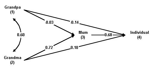
The analysis provided by the program ends here. However, the results cannot be only presented as a list of coefficients, and they are too cumbersome to understand. The results are therefore presented as a path diagram, which has to be constructed from these coefficients.

The convention is for the variables of different layers to line up vertically, and the layers display horizontally from left to right. All variables in the same layers must be connected to each other using curve lines, and labelled with the values of the Partial Correlation Coefficient. All variables are also connected to those in subsequent layers using straight lines, and labelled with the values of the path coefficients. An example (from a different study) may be as follows.

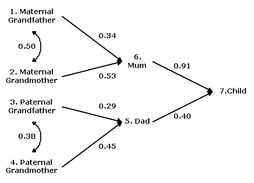
However, if the number of variables involved in the path analysis exceeds 4-5, connecting each variable with every other one becomes unmanageable, and the path diagram becomes cluttered and confused. One way to deal with it is to show only major paths, using statistical significance or an arbitrarily determined size to decide. If only those paths with coefficient values exceeding 0.25, then the path diagram from this example will looks as follows.

References

Pedhazur E. Multiple Regression in Behavioral Research. Explanation and Prediction.( 3rd. ed. 1997) Harcourt Brace College Publishers, Fort Worth, USA. ISBN 0-03-072831-2 . Chapter 18 Structural Equation Models with Observed Variables: Path Analysis. p765-840

ttps://en.wikipedia.org/wiki/Path_analysis_(statistics) Path Analysis by Wikipedia

https://www.thoughtco.com/path-analysis-3026444 Introduction for beginners

https://psych.unl.edu/psycrs/942/q2/path.pdfLecture slides from Umiversity Nebraska Lincoln

Correlation Matrix

Paths Variables Matrix


Data Entry
The correlation matrix :

must have the same numbers of rows and columns, with the value of 1 in the diagonal, and all other cells contain a correlation coefficient.

The path variable matrix

contains variables (column in the correlation matrix) numbers. Numbers in each row represents the variables in a layer or ordered sequence. Each number must not be used more than once.

Please Note : Col and row counts start with 1, so the first col or row is col 1 or row 1