Macroplot plotting is controlled by the macros in the text area provided.
Each macro must occupy its own line. If the first character of a macro is not A-Z, the line will be considered a comment and ignored
The first macro, which is obligatory, initializes the plot. The macro is
Bitmap Initialize width(in pixels), height(in pixels), red(0-255) blue(0-255), green(0-255) transparency(0-255)
Example : Bitmap Initialize 700 500 255 255 255 255 which provides a landscape area 700 pixels wide, 500 pixel high, with white background
The following are default settings when the bitmap is initiated.
Lines are black (0 0 0 255) and 3 pixels in width
Fill color for bars and dots are black (0 0 0 255), and the fill type is set to fill only (1) (see Fill Type)
Dots (circl and square) are set to 5 pixels radius (diameter=11 pixels)
Fonts are set as follows
Font face is set to sans-serif. Serif, sans-serif, and monospace are available to all browsers, user can use any font available to his/her browser
Font size is set to 16 pixels high
Font color, both line and fill are set to black (0 0 0 255), and fill type to 1 (fill only) (see Font Type)
Macros for plotting on the bitmap begin with the keyword Bitmap, and the coordinates are x=number of pixels from the left border and y=number of pixels from the top border
A central plotting area is also defined
By default, at initialization, as 15% from the left and bottom, 5% from right and top
defined by user as Plot Pixels left top right bottom, these being number of pixels from the left and top border
e.g. Plot Pixels 105 25 665 425 would be the same as the default setting for a bitmap of 700 pixels wide and 500 pixels high
The values of the data used in plotting in this central area can be defined as follows
Plot Values left top right bottom, these being the extreme values used in the data
e.g.Plot Values 0 100 10 50 represents x values of 0 on the left to 10 to the right, and y values of 50 at the bottom to 100 to the top
After the values are declared, all plotting in the central area uses macros beginning with the keyword Plot, and the coordinates are the values in the data
Macros
This panel lists and describes all macros used in this version of MacroPlot by Javascript. They are divided into the following sub-panels
Initialization and settings
Plotting areas, coordinates used, and drawing of x and y axis
Drawing lines, bars, dots, text, and other shapes
Initialization
This sub-panel lists those macros that initialized the bitmap, and set the parametrs for drawing
Initialize Plotting
Bitmap Initialize w h r g b t is the first and obligatory macro, which Initializes the bitmap
w and h are width and height of the bitmap in number of pixels. The most common dimensions are
w=700 and h= 500 for landscape orientation
w=500 and h=700 for portrait orientation
Both 500 for square bitmap
r g b t represents red, green, blue and transparency values for the background, each value is 0 for non-existence to 255 for maximum intensity. The most commonly used background is white (255 255 255 255)
For most plotting programs in StatsToDo the macro used is Bitmap Initialize 700 500 255 255 255 255, a landscape orientation with white background
Settings for lines
The settings provide parameters for all subsequent plotting until the parameter is reset
Line Color r g b t sets the line color of red, green, blue and transparency values, each value is 0 for non-existence to 255 for maximum intensity. On initialization of the bitmap, line color is lines is set by default to black (0 0 0 255)
Line Thick p sets the thickness of lines to p pixels. On initialiszation, the default setting is 3 pixels for line thickness
Settings for fills
When bars, dots, arcs and wedges are plotted, the interior of these symbols are called fills, and they are set as follows
Fill Color r g b t sets the filling color of red, green, blue and transparency values, each value is 0 for non-existence to 255 for maximum intensity. On initialization of the bitmap, fill color is lines is set by default to black (0 0 0 255).
Fill Type t sets how the fills are to be used, t can be one of the following
t=0: only the outline, defined by the line parameters, are plotted. Fill is ignored
t=1: only fill is carried out, outline is ignored
t=2: both outline and fill are plotted
When the plot is initialized, the default setting for fill type is t=1
Settings for fonts
These set the font characteristics for text output. Please note: settings for lines and fills for fonts are separate and independent to those for general line and shape plottings
Font Face name sets the font face. The program will accept all fonts supported by the user's border. The 3 fonts accepted by all browsers are serif, sans-serif, and monospace. On initialization, sans-serif is set by default
Font Style s where s can be either normal or bold. On initialization the default setting is bold
Font Size h where h is the height of the text in pixels. On initialization, the default font size is set to 16
Font Thick p where p is the thickness of the outline of the font. On initialization, this is set to p=1
Font LColor r g b t sets the color of the outline of the font. On initialization this is set to black (0 0 0 255)
Font FColor r g b t sets the fill color of the of the font. On initialization this is set to black (0 0 0 255)
Font Color r g b t sets both LColor and FColor to the same color. On initialization this is set to black (0 0 0 255)
Font Type t where t determines which part of the font is drawn, and can be one of the following
t=0: only the outline of the font, defined by the thick and LColor parameter is drawn
t=1: only the fill of the font is drawn
t=2: both outline and fill are drawn
When the plot is initialized, the default setting for Font type is t=1
Please Note: When the bitmap is initialized, the default settings, which are suitable for most situations, are automatically set, so users need not worry about these settings unless he/she has a different preference.
Axis & Coordinates
This sub-panel presents macros that define the plotting areas, and creating the x and y axis for plotting
Drawing on the bitmap
When plotting on the initialized bitmap
the horizontal coordinate x is the number of pixels from the left border
the vertical coordinate y is the number of pixels from the top border
The macro used begins with the keyword Bitmap
Drawing on the plotting area
In most cases, there is a need to draw and label the x and y axis, and drawing coordinates used are the actual values of the data. The macros used for these all begins with the keyword Plot, and are purposes are as follows
Plot Pixels lp tp rp bp defines an area for plotting
lp defines the left border of the plotting area, in the number of pixels from the left border of the bitmap. In most cases this is 15% of the bitmap's width
tp defines the top of the plotting area, in the number of pixels from the top border of the bitmap. In most cases this is 5% of the height
rp defines the right border of the plotting area, in the number of pixels from the left border of the bitmap. In most cases this is 95% of the width (or 5% from the right border of the bitmap)
bp defines the bottom border of the plotting area, in the number of pixels from the top border of the bitmap. In most cases this is 85% of the height (or 15% from the bottom)
An example is that is that, in a landscape orientated bitmap of 700 pixels width and 500 pixel height, Plot Pixels 105 25 665 425 sets the central area for plotting that is 15% from the left and bottom, and 5% from the top and right.
This macro is usually not necessary if the 5%/15% setting suits the user, as this is the default setting when the bitmap is initialized
Plot Values lv tv rv bv defines the data values to be used in plotting
lv is the extreme data value for the horizontal variable x on the left
tv is the extreme data value for the vertical variable y at the top
rv is the extreme data value for horizontal variable x on the right
bv is the extreme data value for the vertical variable y at the bottom
Plot Logx 1 sets the horizontal x axis to the log scale. Normal scale is set on initialization, or reset by Plot Logx 0
Plot Logy 1 sets the vertical y axis to the log scale. Normal scale is set on initialization, or reset by Plot Logy 0
Plot XLabel label distance places the label for the horizontal x axis, below the bottom of the plotting area
lable is a single word text string, using the underscore _ to represent spaces if necessary
space is the number of pixels between the bottom of the plot area and the label text string
Plot YLabel label distance places the label for the vertical y axis, on the left of plotting area
lable is a single word text string, using the underscore _ to represent spaces if necessary
space is the number of pixels between the left of the plot area and the label text string
The quickest and easiest way to draw axis
The following 4 macros are sufficient to draw the x and y axis under most circumstances
Plot XAxis y nsIntv nbIntv len gap line will mark out and numerate the horizontal x axis
y is the y value on which the x axis lie
nsIntv is the number of small intervals between the vertical line marks, 10 to 20 are recommended
nbIntv is the number of big intervals between the numerical scales, 5 to 10 are recommended
len is the length of the mark in pixels, +ve value downwards and negative value upwards. -10 is recommended
gap is the number of pixels between the numerical scaling text and the y value of the axis, +ve values for text below axis and negative value for text above axis. 3 is recommended
Line determines the axis line is drawn, 0 for no line, 1 for line
Plot YAxis x nsIntv nbIntv len gap line will mark out and numerate the vertical y axis
x is the x value on which the y axis lie
nsIntv is the number of small intervals between the horizontal line marks, 10 to 20 are recommended
nbIntv is the number of big intervals between the numerical scales, 5 to 10 are recommended
len is the length of the mark in pixels, +ve value to the right and negative value to the left. 10 is recommended
gap is the number of pixels between the numerical scaling text and the y value of the axis, +ve values for text to the right of axis and negative value for text to the left of axis. -3 is recommended
Line determines the axis line is drawn, 0 for no line, 1 for line
Plot AutoXLogScale y len gap line will mark and numerate the x axis if it is in log scale
The x axis must be set to the log scale by Plot Logx 1. If axis not set to log this macro will abort
y is the y value on which the x axis lie
len is the length of the mark in pixels, +ve value downwards and negative value upwards. -10 is recommended
gap is the number of pixels between the numerical scaling text and the y value of the axis, +ve values for text below axis and negative value for text above axis. 3 is recommended
Line determines the axis line is drawn, 0 for no line, 1 for line
Plot AutoYLogScale x len gap line will mark and numerate the y axis if it is in log scale
The y axis must be set to the log scale by Plot Logy 1. If axis not set to log this macro will abort
x is the x value on which the x axis lie
len is the length of the mark in pixels, +ve value downwards and negative value upwards. -10 is recommended
gap is the number of pixels between the numerical scaling text and the y value of the axis, +ve values for text below axis and negative value for text above axis. 3 is recommended
Line determines the axis line is drawn, 0 for no line, 1 for line
Other methods of drawing axis
Users may wish to draw individual part of the axis, and the following macros can be used
Plot XLine y Draws the horizontal x axis line at the y value y
Plot YLine x Draws the vertical y axis line at the x value y
Plot XMark y begin interval len marks the horizontal x axis with a series of vertical marks
y is the y value where the axis is to be marked
begin is the value for the first mark
interval is the interval between marks
len is the length of the mark line in pixels, +ve downwards, -ve upwards
Plot YMark x start interval len marks the vertical y axis with a series of horizontal marks
x is the x value where the axis is to be marked
start is the value for the first mark
interval is the interval between marks
len is the length of the mark line in pixels, +ve to the right, -ve to the left
Plot XScale y start interval gap writes the numerical scales for the horizontal x axis
y is the y value for the axis
start is the first value to be written
interval is the interval between numerical scales
gap is the space in pixels between the scale text and the axis, +ve for text below axis, -ve for text above axis
The number of decimal points in the scale is the same as that of the interval value
Plot YScale x start interval gap writes the numerical scales for the vertical y axis
x is the x value for the axis
start is the first value to be written
interval is the interval between numerical scales
gap is the space in pixels between the scale text and the axis, +ve for text to the right of axis, -ve for text to the left of axis
The number of decimal points in the scale is the same as that of the interval value
Plot XMarkIntv y interval len marks the horizontal x axis with a series of vertical marks
y is the y value of the axis
interval is the interval between the marks, beginning at 0 and while in range
len is the length of the mark line in pixels, +ve downwards, -ve upwards
Plot YMarkIntv x interval len marks the vertical y axis with a series of horizontal marks
x is the x value of the axis
interval is the interval between the marks, beginning at 0 and while in range
len is the length of the mark line in pixels, +ve to the right, -ve to the left
Plot XScaleIntv y interval gap writes the numerical scales for the horizontal x axis
y is the y value of the axis
interval is the interval between the numerical scales, beginning at 0 and while in range
gap is the space in pixels between the scale text and the axis, +ve for text below axis, -ve for text above axis
The number of decimal points in the scale is the same as that of the interval value
Plot YScaleIntv x interval gap writes the numerical scales for the vertical y axis
x is the x value of the axis
interval is the interval between the numerical scales, beginning at 0 and while in range
gap is the space in pixels between the scale text and the axis, +ve for text to the right of axis, -ve for text to the left of axis
The number of decimal points in the scale is the same as that of the interval value
Drawings
This sub-panel describes those macros that draws the plotting objects. Drawing are performed in two environments
Macros that begins with the keyword Bitmap uses pixel values as coordinates, where x is the number of pixels from the left border, and y the number of pixels from the top border
Macros that begins with the keyword Plot uses actual data values (as defined in the Plot Values lv tv rv bv macro, as coordinates
Drawing lines
The thickness and color of any line drawn is set by the Line macros (see setting sub-panel). The default setting is black line 3 pixels in width
Bitmap Line x1 y1 x2 y2 draws the line from x1y1 to x2y2
x1 and x2 are number of pixels from the left border
y1 and y2 are number of pixels from the top border
Plot Line x1 y1 x2 y2 draws the line from x1y1 to x2y2
x1 and x2 are data values for the horizontal variable x
y1 and y2 are data variables for the vertical variable y
Plot PixLine x y hpix vpix draws a line
x and y are data values for the horizonal x value and verticsl y value. This defines the coordinate at the origin of the line
hpix is the number of pixels horizontally from the origin, +ve value to the right, -ve value to the left
vpix is the number of pixels vertically from the origin, +ve value downwards, -ve value upwards
The line is then drawn between the origin and that defined by hpix and vpix
Drawing bars
The color and thickness of the outline are defined in the Line macro. The color of the fill is defined in the fill color and Fill Type macro. The default setting is black (0 0 0 255) for both line and fill color, and the Fill type is set to 1, only the fill and no outlines. These settings are suitable for most circumstances, but user can change them is so required.
Bitmap Bar x1 y1 x2 y2 draws a bar the corner of which are x1y1 and x2y2. X and y are number of pixels from the left and top border of the bitmap
Plot Bar x1 y1 x2 y2 draws a bar the corner of which are x1y1 and x2y2. X and y are data values as defined in Plot Values lv tv rv bv
Bar Wide w sets the width / height of bars for Plot VBar and Plot HBar
w is the half width of the bar, so a VBar is 2w+1 pixels in width, and HBar is 2w+1 pixels in height
The default value for w is 7 pixels (making width/height of 15 pixels), unless the user changes it
Plot VBar x y1 y2 hshift draws a vertical bar
x is the data value for the horizontal x variable. The is the center of the vertical bar
y1 and y2 are values for the vertical y variable. They define the vertical ends of the bar
hshift is the number of pixels the whole bar is shefted horizontally, +ve value to the left and +ve value to the right. In most cases this is 0 (no shift). However, if there are more than 1 bar in the same position, shifting some of them will avoid the bars overlapping and obscuring each other
The width of the vertical bar is set by default at 7, (width of bar=15 pixels)
Plot HBar x1 x2 y vshift draws a horizontal bar
x1 and x2 are data values for the horizontal x variable. They define the horizontal ends of the bar
y is the value for the vertical y variable, and defines and center of the horizontal bar
vshift is the number of pixels the whole bar is shefted vertically, -ve value upwards and +ve value downwards. In most cases this is 0 (no shift). However, if there are more than 1 bar in the same position, shifting some of them will avoid the bars overlapping and obscuring each other
Theheight of the horizontal bar is set by default at 7, (height of bar=15 pixels)
Drawing dots
There are only 2 dot types, circle and square. If more than 2 tyoes of dats are required, they can be distinguished by the colours of the outline and fill, and by their sizes. Settingsd for dot parameters are in the settings sub-panel
Bitmap Circle x y radius and Bitmap Square x y radius draws a circle or a square dot
x and y are the number of pixels from the left and top border
Radius is in number of pixels. The diameter of the dot is 2Radius+1 pixels
Plot Circle x y radius hshift vshift and Plot Square x y radius hshift vshift draws a circle or a square dot
x and y are the data values of the horizontal x variable and vertical y variable, as defined by Plot Values lv tv rv bv
Radius is in number of pixels. The diameter of the dot is 2Radius+1 pixels
hshift is the number of pixels the dot is shifted horizontally, -ve value to the left, +ve value to the right
vshift is the number of pixels the dot is shifted vertically, -ve value upwards, +ve value downwards
In most cases there is no shift (0 0), but id there are more than 1 dot in the same position, shifting avoids the dots superimposing over and obscuring each other
Dot Radius r sets the radius of the dot in pixels. The diameter of the dot is 2radius+1 pixels. The default radius is 5
Dot Type t where t is either circle or square. The default setting is circle
Plot Dot x y hshift vshift draws the dot, with its parameters (shape size color outline fill) already pre-set
x and y are the data values of the horizontal x variable and vertical y variable, as defined by Plot Values lv tv rv bv
hshift is the number of pixels the dot is shifted horizontally, -ve value to the left, +ve value to the right
vshift is the number of pixels the dot is shifted vertically, -ve value upwards, +ve value downwards
In most cases there is no shift (0 0), but if there are more than 1 dot in the same position, shifting avoids the dots superimposing over and obscuring each other
Drawing text
The color, outline, fill, font, and weight of text are preset (see settings). The default settinfs are sans-sherif, black fill only, and 16pxs high
Bitmap HText x y ha va txt draws text horizontally on the bitmap
x and y are number of pixels fom the left and top borders, and together being the reference coordinate of the text
ha is horizontal adjust
ha=0: the left end of the text is at the x coordinate
ha=1: the center of the text is at the x coordinate
ha=2: the right end of the text is at the x coordinate
va is vertical adjust
va=0: the top of the text is at the y coordinate
va=1: the center of the text is at the x coordinate
va=2: the bottom end of the text is at the x coordinate
txt is the text to be drawn. It must be a single word with no gaps. Spaces can be represented by the underscore _
Plot HText x y ha va txt hshift vshift draws text horizontally on the bitmap
x and y are data values as defined by Plot Values lv tv rv bv, and together being the reference coordinate of the text
ha is horizontal adjust
ha=0: the left end of the text is at the x coordinate
ha=1: the center of the text is at the x coordinate
ha=2: the right end of the text is at the x coordinate
va is vertical adjust
va=0: the top of the text is at the y coordinate
va=1: the center of the text is at the x coordinate
va=2: the bottom end of the text is at the x coordinate
txt is the text to be drawn. It must be a single word with no gaps. Spaces can be represented by the underscore _
hshift is the number of pixels the text is shifted horizontally, -ve value to the left, +ve value to the right
vshift is the number of pixels the text is shifted vertically, -ve value upwards, +ve value downwards
In most cases there is no shift (0 0), but if there are other structures in the same position, shifting avoids the text and structures obscuring each other
Bitmap VText x y ha va txt draws text vertically (90 degrees anticlockwise from horizontal) on the bitmap
x and y are number of pixels fom the left and top borders, and together being the reference coordinate of the text
ha is horizontal adjust
ha=0: the left end of the text is at the x coordinate
ha=1: the center of the text is at the x coordinate
ha=2: the right end of the text is at the x coordinate
va is vertical adjust
va=0: the top of the text is at the y coordinate
va=1: the center of the text is at the x coordinate
va=2: the bottom end of the text is at the x coordinate
txt is the text to be drawn. It must be a single word with no gaps. Spaces can be represented by the underscore _
Plot VText x y ha va txt hshift vshift draws text vertically (90 degrees anticlockwise from horizontal) on the bitmap
x and y are data values as defined by Plot Values lv tv rv bv, and together being the reference coordinate of the text
ha is horizontal adjust
ha=0: the left end of the text is at the x coordinate
ha=1: the center of the text is at the x coordinate
ha=2: the right end of the text is at the x coordinate
va is vertical adjust
va=0: the top of the text is at the y coordinate
va=1: the center of the text is at the x coordinate
va=2: the bottom end of the text is at the x coordinate
txt is the text to be drawn. It must be a single word with no gaps. Spaces can be represented by the underscore _
hshift is the number of pixels the text is shifted horizontally, -ve value to the left, +ve value to the right
vshift is the number of pixels the text is shifted vertically, -ve value upwards, +ve value downwards
In most cases there is no shift (0 0), but if there are other structures in the same position, shifting avoids the text and structures obscuring each other
Other miscellaneous drawings
Bitmap Arc x y radius startDeg endDeg rotate draws an arc.
x and y are number of pixels from the left and top border, and together form the center of the arc
radius is the radius of the arc, in number of pixels
startDeg and endDeg are the degrees (360 degrees in full circle) of the arc
rotate defines the direction of the arc, 0 for clockwise, 1 for anti-clockwise
Bitmap Wedge x y radius startDeg endDeg shift rotate draws a wedge, essentially an arc with lines to the center
x and y are number of pixels from the left and top border, and together form the center of the wedge
radius is the radius of the edge, in number of pixels
startDeg and endDeg are the degrees (360 degrees in full circle) of the wedge
shift is the number of pixels that the wedge is moved centrifugally (away from the center). This is used in pie charts to separate the wedges of the pie
rotate defines the direction of the wedge, 0 for clockwise, 1 for anti-clockwise
Plot Curve a b1 b2 b3 b4 b5 x1 x2 draws a polynomial curve
The curve is y=a + b1x + b2x2 + b3x3 + b4x4 + b5x5. Where higher power is not needed, 0 is used to represent the the coefficient b
The curve is drawn from data value x from x1 to x2
Plot Normal mean sd height draws a normal distribution curve
mean and sd (Standard Deviation) are as in the data horizontal variable variable x
height is the maximum height (where x=mean) of the curve as in the vertical variable y
Color Palettes
Plain Colors
0 0 0 #000000
0 0 63 #00003f
0 0 127 #00007f
0 0 191 #0000bf
0 0 255 #0000ff
0 63 0 #003f00
0 63 63 #003f3f
0 63 127 #003f7f
0 63 191 #003fbf
0 63 255 #003fff
0 127 0 #007f00
0 127 63 #007f3f
0 127 127 #007f7f
0 127 191 #007fbf
0 127 255 #007fff
0 191 0 #00bf00
0 191 63 #00bf3f
0 191 127 #00bf7f
0 191 191 #00bfbf
0 191 255 #00bfff
0 255 0 #00ff00
0 255 63 #00ff3f
0 255 127 #00ff7f
0 255 191 #00ffbf
0 255 255 #00ffff
63 0 0 #3f0000
63 0 63 #3f003f
63 0 127 #3f007f
63 0 191 #3f00bf
63 0 255 #3f00ff
63 63 0 #3f3f00
63 63 63 #3f3f3f
63 63 127 #3f3f7f
63 63 191 #3f3fbf
63 63 255 #3f3fff
63 127 0 #3f7f00
63 127 63 #3f7f3f
63 127 127 #3f7f7f
63 127 191 #3f7fbf
63 127 255 #3f7fff
63 191 0 #3fbf00
63 191 63 #3fbf3f
63 191 127 #3fbf7f
63 191 191 #3fbfbf
63 191 255 #3fbfff
63 255 0 #3fff00
63 255 63 #3fff3f
63 255 127 #3fff7f
63 255 191 #3fffbf
63 255 255 #3fffff
127 0 0 #7f0000
127 0 63 #7f003f
127 0 127 #7f007f
127 0 191 #7f00bf
127 0 255 #7f00ff
127 63 0 #7f3f00
127 63 63 #7f3f3f
127 63 127 #7f3f7f
127 63 191 #7f3fbf
127 63 255 #7f3fff
127 127 0 #7f7f00
127 127 63 #7f7f3f
127 127 127 #7f7f7f
127 127 191 #7f7fbf
127 127 255 #7f7fff
127 191 0 #7fbf00
127 191 63 #7fbf3f
127 191 127 #7fbf7f
127 191 191 #7fbfbf
127 191 255 #7fbfff
127 255 0 #7fff00
127 255 63 #7fff3f
127 255 127 #7fff7f
127 255 191 #7fffbf
127 255 255 #7fffff
191 0 0 #bf0000
191 0 63 #bf003f
191 0 127 #bf007f
191 0 191 #bf00bf
191 0 255 #bf00ff
191 63 0 #bf3f00
191 63 63 #bf3f3f
191 63 127 #bf3f7f
191 63 191 #bf3fbf
191 63 255 #bf3fff
191 127 0 #bf7f00
191 127 63 #bf7f3f
191 127 127 #bf7f7f
191 127 191 #bf7fbf
191 127 255 #bf7fff
191 191 0 #bfbf00
191 191 63 #bfbf3f
191 191 127 #bfbf7f
191 191 191 #bfbfbf
191 191 255 #bfbfff
191 255 0 #bfff00
191 255 63 #bfff3f
191 255 127 #bfff7f
191 255 191 #bfffbf
191 255 255 #bfffff
255 0 0 #ff0000
255 0 63 #ff003f
255 0 127 #ff007f
255 0 191 #ff00bf
255 0 255 #ff00ff
255 63 0 #ff3f00
255 63 63 #ff3f3f
255 63 127 #ff3f7f
255 63 191 #ff3fbf
255 63 255 #ff3fff
255 127 0 #ff7f00
255 127 63 #ff7f3f
255 127 127 #ff7f7f
255 127 191 #ff7fbf
255 127 255 #ff7fff
255 191 0 #ffbf00
255 191 63 #ffbf3f
255 191 127 #ffbf7f
255 191 191 #ffbfbf
255 191 255 #ffbfff
255 255 0 #ffff00
255 255 63 #ffff3f
255 255 127 #ffff7f
255 255 191 #ffffbf
255 255 255 #ffffff
Color Palletes
Table of colors used on this web site
255 255 255 #ffffff
224 224 224 #e0e0e0
128 128 128 #808080
128 0 0 #800000
255 0 0 #ff0000
96 48 96 #603060
48 16 64 #301040
96 96 160 #6060a0
160 160 96 #a0a060
160 160 0 #a0a000
153 191 164 #99bfa4
160 160 96 #a0a060
97 24 0 #611800
204 63 200 #cc3fc8
224 224 224 #e0e0e0
Patterns of complementary colors
A
105 93 70 #695d46
255 113 44 #ff712c
207 194 145 #cfc291
161 232 217 #a1e8d9
255 246 197 #fff6c5
B
115 0 70 #730046
201 60 0 #c93c00
232 136 1 #e88801
255 194 0 #ffc200
191 187 17 #bfbb11
C
97 24 0 #611800
140 115 39 #8c7327
71 164 41 #47a429
153 191 164 #99bfa4
242 239 189 #f2efbd
D
20 87 110 #14576e
140 33 90 #8c215a
230 133 38 #e68526
195 102 163 #c366a3
242 207 242 #f2cff2
E
64 1 1 #400101
48 115 103 #307367
96 166 133 #60a685
242 236 145 #f2ec91
229 249 186 #e5f9ba
F
55 89 21 #375915
166 60 60 #a63c3c
115 108 73 #736c49
166 157 129 #a69d81
242 224 201 #f2e0c9
G
115 36 94 #73245e
166 69 33 #a64521
217 182 78 #d9b64e
242 218 145 #f2da91
242 242 242 #f2f2f2
H
255 77 0 #ff4d00
102 87 71 #665747
125 179 0 #7db300
153 138 122 #998a7a
217 195 98 #d9c362
I
128 0 38 #800026
128 128 83 #808053
92 153 122 #5c997a
163 204 143 #a3cc8f
255 230 153 #ffe699
Explanations
CUSUM Generally
CUSUM is a set of statistical procedures used in quality control. CUSUM stands for Cumulative Sum of Deviations.
In any ongoing process, be it manufacture or delivery of services and products, once the process is established and running, the outcome should be stable and within defined limits near a benchmark. The situation is said to be In Control
When things go wrong, the outcomes depart from the defined benchmark. The situation is then said to be Out of Control
In some cases, things go catastrophically wrong, and the outcomes departure from the benchmark in a dramatic and obvious manner, so that investigation and remedy follows. For example, the gear in an engine may fracture, causing the machine to seize. An example in health care is the employment of an unqualified fraud as a surgeon, followed by sudden and massive increase in mortality and morbidity.
The detection of catastrophic departure from the benchmark is usually by the Shewhart Chart, not covered on this site. Usually, some statistically improbable outcome, such as two consecutive measurements outside 3 Standard Deviations, or 3 consecutive measurements outside 2 Standard Deviations, is used to trigger an alarm that all is not well.
In many instances however, the departures from outcome benchmark are gradual and small in scale, and these are difficult to detect. Examples of this are changes in size and shape of products caused by progressive wearing out of machinery parts, reduced success rates over time when experienced staff are gradually replaced by novices in a work team, increases in client complaints to a service department following a loss of adequate supervision.
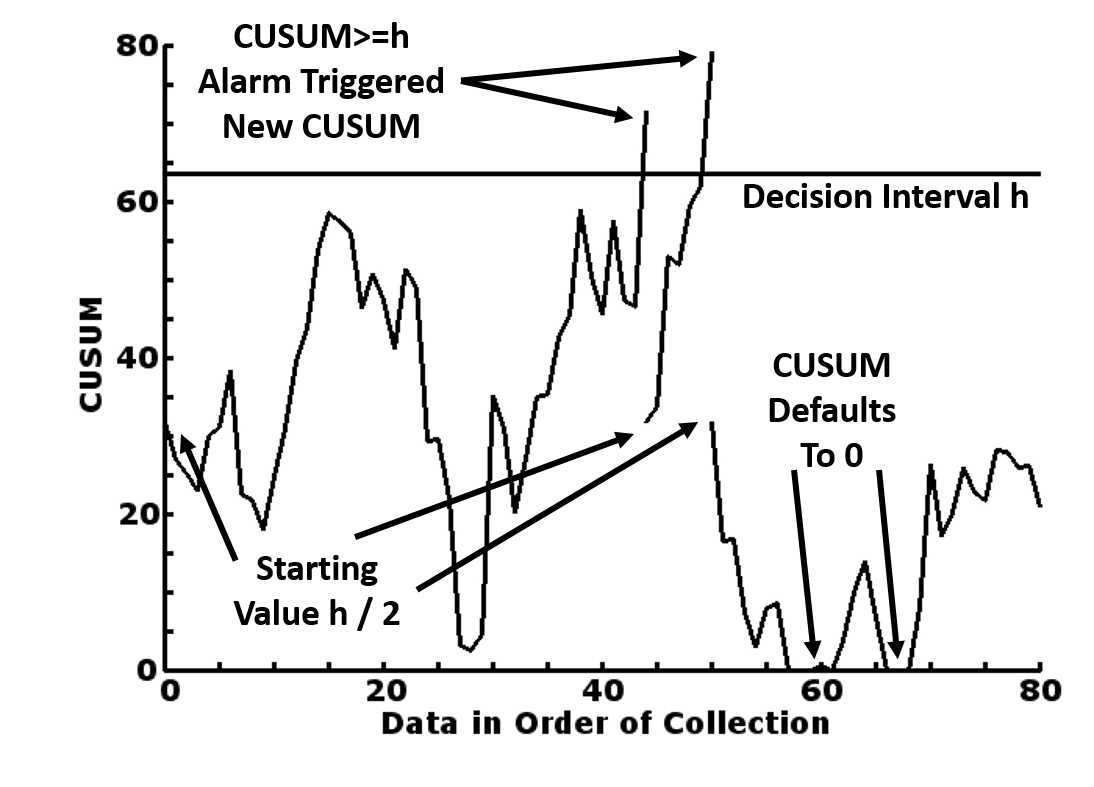
CUSUM is a statistical process of sampling outcome, and summing departures from benchmarks. When the situation is in control, the departures caused by random variations cancel each other numerically. In the out of control situation, departures from benchmark tend to be unidirectional, so that the sum of departures accumulates until it becomes statistically identifiable. The general layout of a CUSUM chart is as shown in the plot to the right
Terminology
In control describe the situation when everything is going according to plan, and the measurements being monitored are within the benchmark.
Out of control is the situation CUSUM is designed to detect, when the measurements drift outside of the benchmark
Average run length (ARL) is the estimated number of continuous observations before a false alarm is triggered. It is equivalent to the false positive rate or the Type I Error. A false positive rate of 1% (p=0.01) is the same as ARL=100.
The ARL is usually set in a balance between the need for investigation and intervention when things go wrong and the inconvenience and cost of a false alarm. For example, if the sampling rate is 5 a day, and the requirement is that a false alarm does not occur more frequently than every 20 days, then the ARL = 5x20 = 100
The CUSUM is designed to be a one tail algorithm, to test for departure from the benchmark upwards or downwards, but not both. If the user wishes to have a two tail test for both at the same time, then he/she needs to use two CUSUMs, one for each tail, but the ARL for each should be half of that required for the one tail situation.
Data is a vector (array) of values obtained during monitoring that are used to calculate the CUSUM
Terms the user can control, but is usually set in default
Model sets the initial value of CUSUM in a run, which determines how rapidly the out of control situation can be detected if it exists already. The more rapid the response will of course lead to a greater risk of a false alarm. The 3 options are
F for Fast Initial Resposnse (FIR), where the initial CUSUM value is set at half of the Decision Interval (h). This is the default option, as recommended by Hawkin's textbook
Z for zero (0), where the initial CUSUM value is set to 0. This can be used if the user is certain that the situation is in control initially, and wish to avoid an early false alarm
S is for steady state, used when the CUSUM value is supposed to be from the end of a previous CUSUM which has just ended, and the value can be set by the user. S is usually not offered in StatsToDo as this requires the user to alter the algorithm to set an initial value
Winsorization is a statistical process whereby unexpected outliers with extreme values are modified before they are used for calculating CUSUM. Winsorization is not provided in StatsToDo, and users will need to manually modify extreme outlier values before analysis if they should choose to do so.
Terms for results produced by the algorithm
Reference Value (k) is used to adjust the value of the CUSUM and control the proliferation of its variance. It is used in all subsequent calculations, but need not be attended to by the user
Decision Interval (h) the the value of the CUSUM which should trigger an alarm that the out of control situation has been detected.
CUSUM values is calculated from the data using the reference value (k). It is usually stored in a vector, and used for plotting.
CUSUM programs available on StatsToDo
The following programs are available as individual pages on this site
This page is for CUSUM for measurements with Inverse Gaussian distribution
CUSUM for Inverse Gaussian Distribution
All unidirectional measurements are ratios against a known standard, and have positve values. In most cases, the range of measurement is sufficiently far from 0, and the variability sufficiently narrow that the errors incurred by assuming the normal distribution is trivial, and statistical analysis can be carried out with that assumption.
When the values of measurements are close to zero (0), the distribution becomes skewed, as values cannot be less than or equals to zero(0). In many cases, the distribution becomes approximately exponential (with a longer rignt sided tail), and the logarithm of the values are usually assumed to be normally distributed.
When the values are very close to zero (0), and the variations wide, the assumtion of normal distribution (even using logarithmic transformation) becomes invalid, as the probability curve becomes skewed with the mode near the lower values and a long tail for the higher values.
An example of this is in time measurements. When we consider the age of pregnant women, the range is between 20-40 years, with the mode near the mean. The skew is so minor that in most cases age of the mother can be treated as normally distributed values.
However, if we consider the duration of labour, the range is from within a few minutes to over 24 hours, with most women delivered between 4-8 hours. The mode is therefore near the lower values, and there is a long tail of higher values. Statistical analysis based on the assumtion of normality will likely lead to misinterpretations.
Dealing with skewed data
A set of skewed data can be transformed, so that its distribution become closer to normal distribution.
The simplest method is to rank the values, and assume that the ranks are normally distributed. However, the same measurement may have a different rank in another set of data, so interpretations becomes difficult.
The common approach is to use log or square root transformation, as these stretches the intervals amongst the lower values and shrink the intervals of the higher values.
For more complex skews, the Box Cox transformation can be used. The data are transformed, the analysis assumes normal distribution, and the results reverse transformed to the original units.
If transformation is considered inappropriate or may introduce additional errors, the skewed data is accepted as having an inverse Gaussian distribution and analysed as such
CUSUM for the Inverse Gaussian Distribution
When the data is a continuous measurement of all positive values, and has a skew, the Inverse Gaussian distribution is the most appropriate model to use for CUSUM, as the model allows a precise prediction of what the data should be.
Details of how the analysis is done and the results are describer in the R Code panel. Conceptually, the algorithm is as follows
Before monitoring begins, a set of reference data must be obtained to create the model, so that the central location (mu μ) and the skew (lambda λ) can be estimated. These become the in control mu and lambda.
The out of control location (mu) is then nominated.
With the in and out of control parameters, and the average run length, the reference value (k) and decision interval h can be computed.
CUSUM can then be calculated and plotted using monitoring data.
Details of how the analysis is done and the results are describer in the R code panel
Plotting CUSUM
Each CUSUM value (CUSUMn) is the previous CUSUM value (CUSUNn-1, plus the current value (v), corrected by the Reference value (k)
CUSUMn = CUSUMn-1 + v - k
If CUSUM crosses the zero value (0) it is truncated to 0
The CUSUM values are plotted sequentially. An alarm is triggered when CUSUM crosses the Decision Interval (h)
Please note: Plotting for CUSUM on this page is provided both using R codes, and Javascript plotting
References
CUSUM : Hawkins DM, Olwell DH (1997) Cumulative sum charts and charting for
quality improvement. Springer-Verlag New York. ISBN 0-387-98365-1 p 47-74, 147-148
Hawkins DM (1992) Evaluation of average run lengths of cumulative sum charts for an arbitrary data distribution. Journal Communications in Statistics - Simulation and Computation Volume 21, - Issue 4 Pages 1001-1020
The example is a made up one to demonstrate the numerical process, and the data is generated by the computer. It purports to be from a quality control exercise in the outpatient clinic, using the patient waiting time between arrival and being attended to as the quality indicator.
After much organization and training, the initial benchmark has been achieved, that patients do not have to wait much more than 20 minutes between arrival and being attended to. CUSUM is then established to monitor that this standard is maintained.
With time, experienced and trained staff leave and replaced by the less experienced and trained. The standard may then deteriorate, resulting in progressively longer waiting time for patients.
We would like to trigger an alarm to carry out re-training and reorganization when the waiting time doubled to that of the bench mark.
As training and re-organization is disruptive to services, we set the average run length (ARL) to 100. If we sample one waiting time per clinic session, the false alarm rate should be no more frequent than 100 clinic sessions.
Step 0: Estimate In Control mu (μ) and lambda (λ)
# Step 0: before monitoring, establish in control mu and lambda
refData <- c(7.5, 4, 5.5, 9, 7, 16, 3.5, 17.5, 11.5, 14.5, 11, 7.5, 12.5, 11, 6.5, 8, 9, 6.5,
             20, 12, 13, 10, 11.5, 13, 7.5, 11, 2, 14.5, 17, 10, 20.5, 9, 2.5, 7, 18.5, 6, 3.5,
             3, 13, 17, 7, 10.5, 10.5, 6.5, 24.5, 6, 10.5, 5.5, 8.5, 17)
#install.packages("goft")    # if not already installed
library(goft)
ig_fit(refData)              # fitting an inverse Gaussian distribution to refData
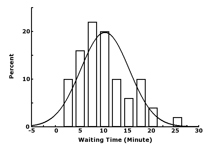
Step 0 is undertaken during the planning stage. We collect waiting time (in minutes closest 0.5 minutes) from 50 patients. It can be seen from the plot to the right that, when compared with the theoretical normal distribution curve, the data is skewed to the left with a long right tail, and the 95% confidence interval on the left would include the impossible negative values. This is typical of the Inverse Gaussian Distribution.
We calculate the central location (mu) and skew(λ), which describe the in control charactersitcs based on the Inverse Gaussian Distribution. The results are:
       Inverse Gaussian MLE
mu                  10.32000
lambda              28.95172
Step 1: Define CUSUM Parameters
# Step 1 Input parameters
inControlMu = 10
inControlLambda = 29
outOfControlMu = 20
arl = 100
theModel = "F"   #F for FIR,   Z for zero, S for steady state
Step 1 estimates k and h, using in control μ and λ, out of control μ and the arl.
The model has 3 options, which sets the first value of the CUSUM
F means Fast Initial Response, where the initial CUSUM value is set at half of the Decision Interval h. The rationale is that, if the situation is in control then CUSUM will gradually drift towards zero, but if the situation is already out of control, an alarm would be triggered early. The down side is that a false alarm is slightly more likely early on in the monitoring. As FIR is recommended by Hawkins, it is set as the default option
Z is for zero, and CUSUM starts at the baseline value of 0. This will lower the risk of false alarm in the early stages of monitoring, but will detect the out of control situation slower if it already exists at the begining.
S is for steady state, intended for when monitoring is already ongoing, and a new plot is being constructed. The CUSUM starts at the value when the previous chart ends.
Each model will make minor changes to the value of the decision interval h. The setting of the initial values is mostly intended to determine how quickly an alarm can be triggered if the out of control situation exists from the beginning.
Step 2: Calculate Reference Value (k) and Decision Interval (h)
# Step 2: Calculate k and h
#install.packages("CUSUMdesign")   # if not already installed
library(CUSUMdesign)
result <- getH(distr=6, ICmean=inControlMu, IClambda=inControlLambda, OOCmean=outOfControlMu,
               ARL=arl, type=theModel)
k = result$ref
h = result$DI
if(outOfControlMu<inControlMu)
{
  h = -h
}
cat("Reference Value k=",k,"\tDecision Interval h=", h, "\n")
result is the object that contains the results of the analysis. The result required for this program are the reference value k and decision interval h. Please note that h is calculated as a positive value. If the CUSUM is designed to detect a decrease from in control value, then h needs to be changed to a negative value.
The results are as follows
Reference Value k= 13.33333 Decision Interval h= 22.07419
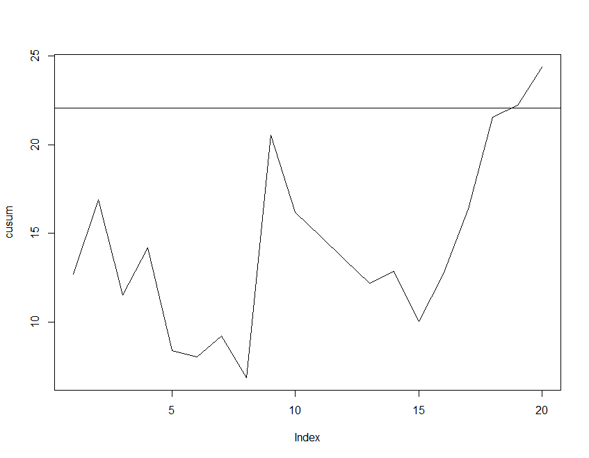
Step 3: CUSUM Plot
Step 3 is divided into 2 parts. Step 3a calculates the cusum vector, and 3b plots the vector and h in a graph.
#Step 3a: Calculate CUSUM. dat is the vector of waiting time
dat=c(15, 17.5, 8, 16, 7.5, 13, 14.5, 11, 27, 9, 12, 12, 12, 14, 10.5, 16, 17, 18.5, 14, 15.5)
cusum <- vector()
cusumValue = 0
if(theModel=="F")
{
  cusumValue = h / 2
}
for(i in 1 : length(dat))
{
  cusumValue = cusumValue + dat[i] - k
  #print(cusumValue)
  if(outOfControlMu>inControlMu) # Up
  {
    if(cusumValue<0)
    {
      cusumValue = 0
    }
  }
  else                               # down
  {
    if(cusumValue>0)
    {
      cusumValue = 0
    }
  }
  cusum[i] = cusumValue
}
cusum
The vector dat contains the waiting time values to be monitored. The resulting cusum vector is
# Step 3b: Plot the cusum vector and h
plot(cusum,type="l")
abline(h=h)
In step 3b, the first line plots the cusum vector, and the second line the decision interval h. The result plot is shown to the right.
Step 4: (Optional) Exporting results
# Step 4: Optional export of results
#myDataFrame <- data.frame(dat,cusum)       #combine dat and cusum to dataframe
#myDataFrame                                #display dataframe
#write.csv(myDataFrame, "CusumInvGauss.csv")   # write dataframe to .csv file
Step 4 is optional, and in fact commented out, and included as a template only. Each line can be activated by removing the #
The first line places the two vectors, dat and cusum together into a dataframe
The second line displays the data, along with row numbers, in the console, which can then be copied and pasted into other applications for further processing
The third line saves the dataframe as a comma delimited .csv file. This is needed if the data is too large to handle by copy and paste from the console.
Javascript Plot
Comments on Plot
The Javascript plot uses MacroPlot to produce the CUSUM plot, using the same parameters as that in the R code.
The parameters are:
k and h are as produced in R
The starting CUSUM value is 0 for Zero start (Model Z), h/2 for FIR (Model Z), and any nominated value for Steady State (Model S). From the default example data, with model Z, the starting value = 87.978 / 2 = 43.989
In the resulting plot:
The x axis is the sequence of observations
The y axis is CUSUM, where CUSUMn = CUSUMn-1 + SD2 - k, truncated to zero (0) if it crosses the zero value
The horizontal line represents the Decision Interval (h)
The example parameters and data are the same as that used in the R codes, and the plot should appear almost identical to that produced by R, with minor ronding errors
In this version, Parameters for calculations of k and h, and the input values, are in Standard Deviations (SD). The k and h values calculated, as well as the CUSUM values to be plotted, are in Variance unit. These format complies with that from the R package.
CUSUM Plot
Data:
Parameters are as calculated in R
Starting CUSUM value=0 for model Z
Starting CUSUM value=h/2 for model F
Reference Value (k)
Decision Interval (h)
Starting CUSUM Value

 Step 0 is undertaken during the planning stage. We collect waiting time (in minutes closest 0.5 minutes) from 50 patients. It can be seen from the plot to the right that, when compared with the theoretical normal distribution curve, the data is skewed to the left with a long right tail, and the 95% confidence interval on the left would include the impossible negative values. This is typical of the Inverse Gaussian Distribution.